Challenge 3 Instructions

challenge_3

animal_weights

eggs

australian_marriage

usa_households

sce_labor

Tidy Data: Pivoting

Author

Kevin Martell Luya

Published

April 21, 2023

Code

library(tidyverse)
library(readxl)
library(lattice)

knitr::opts_chunk$set(echo = TRUE, warning=FALSE, message=FALSE)

Challenge Overview

Today’s challenge is to:

read in a data set, and describe the data set using both words and any supporting information (e.g., tables, etc)
identify what needs to be done to tidy the current data
anticipate the shape of pivoted data
pivot the data into tidy format using pivot_longer

Read in data

Read in one (or more) of the following datasets, using the correct R package and command.

animal_weights.csv ⭐
eggs_tidy.csv ⭐⭐ or organiceggpoultry.xls ⭐⭐⭐
australian_marriage*.xls ⭐⭐⭐
USA Households*.xlsx ⭐⭐⭐⭐
sce_labor_chart_data_public.xlsx 🌟🌟🌟🌟🌟

Briefly describe the data

Describe the data, and be sure to comment on why you are planning to pivot it to make it “tidy”

Anticipate the End Result

The first step in pivoting the data is to try to come up with a concrete vision of what the end product should look like - that way you will know whether or not your pivoting was successful.

One easy way to do this is to think about the dimensions of your current data (tibble, dataframe, or matrix), and then calculate what the dimensions of the pivoted data should be.

Suppose you have a dataset with \(n\) rows and \(k\) variables. In our example, 3 of the variables are used to identify a case, so you will be pivoting \(k-3\) variables into a longer format where the \(k-3\) variable names will move into the names_to variable and the current values in each of those columns will move into the values_to variable. Therefore, we would expect \(n * (k-3)\) rows in the pivoted dataframe!

Example: find current and future data dimensions

Lets see if this works with a simple example.

Code

df<-tibble(country = rep(c("Mexico", "USA", "France"),2),
           year = rep(c(1980,1990), 3), 
           trade = rep(c("NAFTA", "NAFTA", "EU"),2),
           outgoing = rnorm(6, mean=1000, sd=500),
           incoming = rlogis(6, location=1000, 
                             scale = 400))
df

# A tibble: 6 × 5
  country  year trade outgoing incoming
  <chr>   <dbl> <chr>    <dbl>    <dbl>
1 Mexico   1980 NAFTA     909.    -511.
2 USA      1990 NAFTA     491.    1248.
3 France   1980 EU       1133.    1311.
4 Mexico   1990 NAFTA    1190.    1417.
5 USA      1980 NAFTA     807.    1726.
6 France   1990 EU       1139.     848.

Code

#existing rows/cases
nrow(df)

[1] 6

Code

#existing columns/cases
ncol(df)

[1] 5

Code

#expected rows/cases
nrow(df) * (ncol(df)-3)

[1] 12

Code

# expected columns 
3 + 2

[1] 5

Or simple example has \(n = 6\) rows and \(k - 3 = 2\) variables being pivoted, so we expect a new dataframe to have \(n * 2 = 12\) rows x \(3 + 2 = 5\) columns.

Challenge: Describe the final dimensions

Document your work here.

Any additional comments?

Pivot the Data

Now we will pivot the data, and compare our pivoted data dimensions to the dimensions calculated above as a “sanity” check.

Example

Code

df<-pivot_longer(df, col = c(outgoing, incoming),
                 names_to="trade_direction",
                 values_to = "trade_value")
df

# A tibble: 12 × 5
   country  year trade trade_direction trade_value
   <chr>   <dbl> <chr> <chr>                 <dbl>
 1 Mexico   1980 NAFTA outgoing               909.
 2 Mexico   1980 NAFTA incoming              -511.
 3 USA      1990 NAFTA outgoing               491.
 4 USA      1990 NAFTA incoming              1248.
 5 France   1980 EU    outgoing              1133.
 6 France   1980 EU    incoming              1311.
 7 Mexico   1990 NAFTA outgoing              1190.
 8 Mexico   1990 NAFTA incoming              1417.
 9 USA      1980 NAFTA outgoing               807.
10 USA      1980 NAFTA incoming              1726.
11 France   1990 EU    outgoing              1139.
12 France   1990 EU    incoming               848.

Yes, once it is pivoted long, our resulting data are \(12x5\) - exactly what we expected!

Challenge: Pivot the Chosen Data

Document your work here. What will a new “case” be once you have pivoted the data? How does it meet requirements for tidy data?

It is evident that certain columns derive from another ( percentages and total columns which can be obtained from the other columns.We also notice that there are rows with empty values and rows with strings “<> (Total)”. Let’s remove them and keep it simple with essential data.

Code

data <- read_excel("_data/australian_marriage_law_postal_survey_2017_-_response_final.xls",
           sheet="Table 2",
           skip=7,
           col_names = c("DISTRICT","YES","_trash","NO",rep("_trash",6),"RESPONSE_NOT_CLEAR","_trash","NO_RESPONSE",rep("_trash",3)))%>%
  select(!contains("_trash"))%>%
  drop_na(DISTRICT)%>%
  head(-7)%>%
  filter(!str_detect(DISTRICT,"(Total)"))


data

# A tibble: 159 × 5
   DISTRICT                    YES    NO RESPONSE_NOT_CLEAR NO_RESPONSE
   <chr>                     <dbl> <dbl>              <dbl>       <dbl>
 1 New South Wales Divisions    NA    NA                 NA          NA
 2 Banks                     37736 46343                247       20928
 3 Barton                    37153 47984                226       24008
 4 Bennelong                 42943 43215                244       19973
 5 Berowra                   48471 40369                212       16038
 6 Blaxland                  20406 57926                220       25883
 7 Bradfield                 53681 34927                202       17261
 8 Calare                    54091 35779                285       25342
 9 Chifley                   32871 46702                263       28180
10 Cook                      47505 38804                229       18713
# … with 149 more rows

Next, let’s add a new column called Division and set each row value according to the District division name until we find a new one. Then we repeat the process of setting the District divisions name to the rows that are below.

Code

data <-data %>%
  mutate(DIVISION = case_when(
    str_detect(DISTRICT, "Divisions") ~ DISTRICT,
    TRUE ~ NA_character_ ))%>%
  fill(DIVISION, .direction = "down") %>%
  filter(!str_detect(DISTRICT, "Division"))

# remove Australia
data <- filter(data, !str_detect(DISTRICT, "Australia"))
data

# A tibble: 150 × 6
   DISTRICT    YES    NO RESPONSE_NOT_CLEAR NO_RESPONSE DIVISION                
   <chr>     <dbl> <dbl>              <dbl>       <dbl> <chr>                   
 1 Banks     37736 46343                247       20928 New South Wales Divisio…
 2 Barton    37153 47984                226       24008 New South Wales Divisio…
 3 Bennelong 42943 43215                244       19973 New South Wales Divisio…
 4 Berowra   48471 40369                212       16038 New South Wales Divisio…
 5 Blaxland  20406 57926                220       25883 New South Wales Divisio…
 6 Bradfield 53681 34927                202       17261 New South Wales Divisio…
 7 Calare    54091 35779                285       25342 New South Wales Divisio…
 8 Chifley   32871 46702                263       28180 New South Wales Divisio…
 9 Cook      47505 38804                229       18713 New South Wales Divisio…
10 Cowper    57493 38317                315       25197 New South Wales Divisio…
# … with 140 more rows

Let’s pivot the data to get all the response types in one column per district with its respective counts

Code

data_longe <- pivot_longer(
  data,
  cols = YES:NO_RESPONSE,
  names_to = "Response",
  values_to = "Count"
 
)
data_longe

# A tibble: 600 × 4
   DISTRICT  DIVISION                  Response           Count
   <chr>     <chr>                     <chr>              <dbl>
 1 Banks     New South Wales Divisions YES                37736
 2 Banks     New South Wales Divisions NO                 46343
 3 Banks     New South Wales Divisions RESPONSE_NOT_CLEAR   247
 4 Banks     New South Wales Divisions NO_RESPONSE        20928
 5 Barton    New South Wales Divisions YES                37153
 6 Barton    New South Wales Divisions NO                 47984
 7 Barton    New South Wales Divisions RESPONSE_NOT_CLEAR   226
 8 Barton    New South Wales Divisions NO_RESPONSE        24008
 9 Bennelong New South Wales Divisions YES                42943
10 Bennelong New South Wales Divisions NO                 43215
# … with 590 more rows

As a result we pivoted the dataset, but one step is missing if we want to visualize a barchat. Let’s mutate Responses and get the 4 categories by using factor.

Code

data_visualize <- data_longe%>%
  mutate(Response = factor(Response))

summary(data_visualize)

   DISTRICT           DIVISION                       Response       Count      
 Length:600         Length:600         NO                :150   Min.   :  106  
 Class :character   Class :character   NO_RESPONSE       :150   1st Qu.: 9913  
 Mode  :character   Mode  :character   RESPONSE_NOT_CLEAR:150   Median :25477  
                                       YES               :150   Mean   :26677  
                                                                3rd Qu.:40019  
                                                                Max.   :89590

Code

barchart( Count ~ Response , group = DIVISION , data = data_visualize)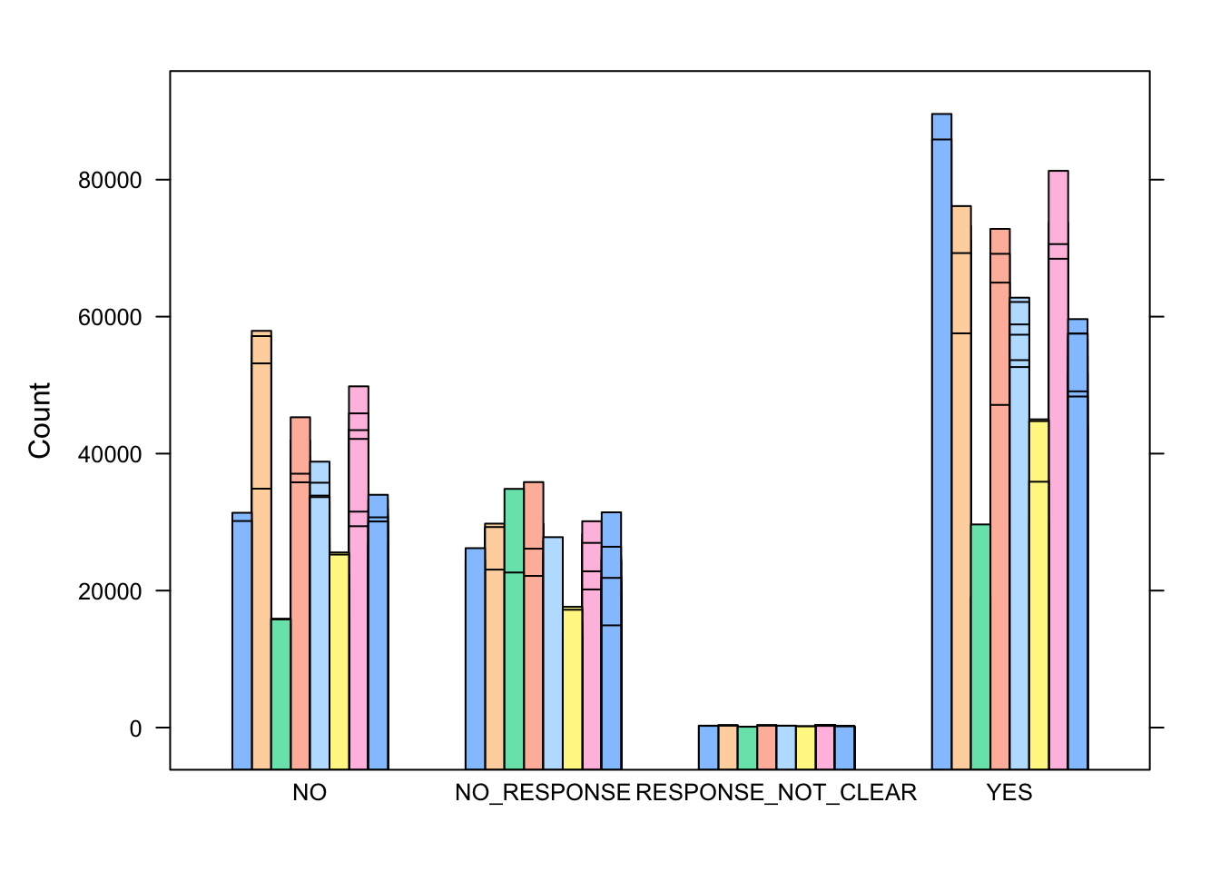

This is the final visualization after using pivoting longe.