library(tidyverse)
library(ggplot2)
library(here)
library(ggthemes)

knitr::opts_chunk$set(echo = TRUE, warning=FALSE, message=FALSE)
Challenge 7 Instructions
challenge_7
hotel_bookings
australian_marriage
air_bnb
eggs
abc_poll
faostat
usa_households
Visualizing Multiple Dimensions
Challenge Overview
Today’s challenge is to:
- read in a data set, and describe the data set using both words and any supporting information (e.g., tables, etc)
- tidy data (as needed, including sanity checks)
- mutate variables as needed (including sanity checks)
- Recreate at least two graphs from previous exercises, but introduce at least one additional dimension that you omitted before using ggplot functionality (color, shape, line, facet, etc) The goal is not to create unneeded chart ink (Tufte), but to concisely capture variation in additional dimensions that were collapsed in your earlier 2 or 3 dimensional graphs.
- Explain why you choose the specific graph type
- If you haven’t tried in previous weeks, work this week to make your graphs “publication” ready with titles, captions, and pretty axis labels and other viewer-friendly features
R Graph Gallery is a good starting point for thinking about what information is conveyed in standard graph types, and includes example R code. And anyone not familiar with Edward Tufte should check out his fantastic books and courses on data visualizaton.
(be sure to only include the category tags for the data you use!)
Read in data
Read in one (or more) of the following datasets, using the correct R package and command.
- eggs ⭐
- abc_poll ⭐⭐
- australian_marriage ⭐⭐
- hotel_bookings ⭐⭐⭐
- air_bnb ⭐⭐⭐
- us_hh ⭐⭐⭐⭐
- faostat ⭐⭐⭐⭐⭐
airb<-here("posts","_data","AB_NYC_2019.csv") %>%
  read_csv()
airb
# A tibble: 48,895 × 16
id name host_id host_…¹ neigh…² neigh…³ latit…⁴ longi…⁵ room_…⁶ price
<dbl> <chr> <dbl> <chr> <chr> <chr> <dbl> <dbl> <chr> <dbl>
1 2539 Clean & … 2787 John Brookl… Kensin… 40.6 -74.0 Privat… 149
2 2595 Skylit M… 2845 Jennif… Manhat… Midtown 40.8 -74.0 Entire… 225
3 3647 THE VILL… 4632 Elisab… Manhat… Harlem 40.8 -73.9 Privat… 150
4 3831 Cozy Ent… 4869 LisaRo… Brookl… Clinto… 40.7 -74.0 Entire… 89
5 5022 Entire A… 7192 Laura Manhat… East H… 40.8 -73.9 Entire… 80
6 5099 Large Co… 7322 Chris Manhat… Murray… 40.7 -74.0 Entire… 200
7 5121 BlissArt… 7356 Garon Brookl… Bedfor… 40.7 -74.0 Privat… 60
8 5178 Large Fu… 8967 Shunic… Manhat… Hell's… 40.8 -74.0 Privat… 79
9 5203 Cozy Cle… 7490 MaryEl… Manhat… Upper … 40.8 -74.0 Privat… 79
10 5238 Cute & C… 7549 Ben Manhat… Chinat… 40.7 -74.0 Entire… 150
# … with 48,885 more rows, 6 more variables: minimum_nights <dbl>,
# number_of_reviews <dbl>, last_review <date>, reviews_per_month <dbl>,
# calculated_host_listings_count <dbl>, availability_365 <dbl>, and
# abbreviated variable names ¹host_name, ²neighbourhood_group,
# ³neighbourhood, ⁴latitude, ⁵longitude, ⁶room_typeBriefly describe the data
AB_NYC_2019.csv contains listing data about rental places in New York. It would be interesting analyzing this data which comes from the concept of share economy.
Tidy Data (as needed)
Is your data already tidy, or is there work to be done? Be sure to anticipate your end result to provide a sanity check, and document your work here.
ggplot(airb,aes(minimum_nights))+
  geom_histogram()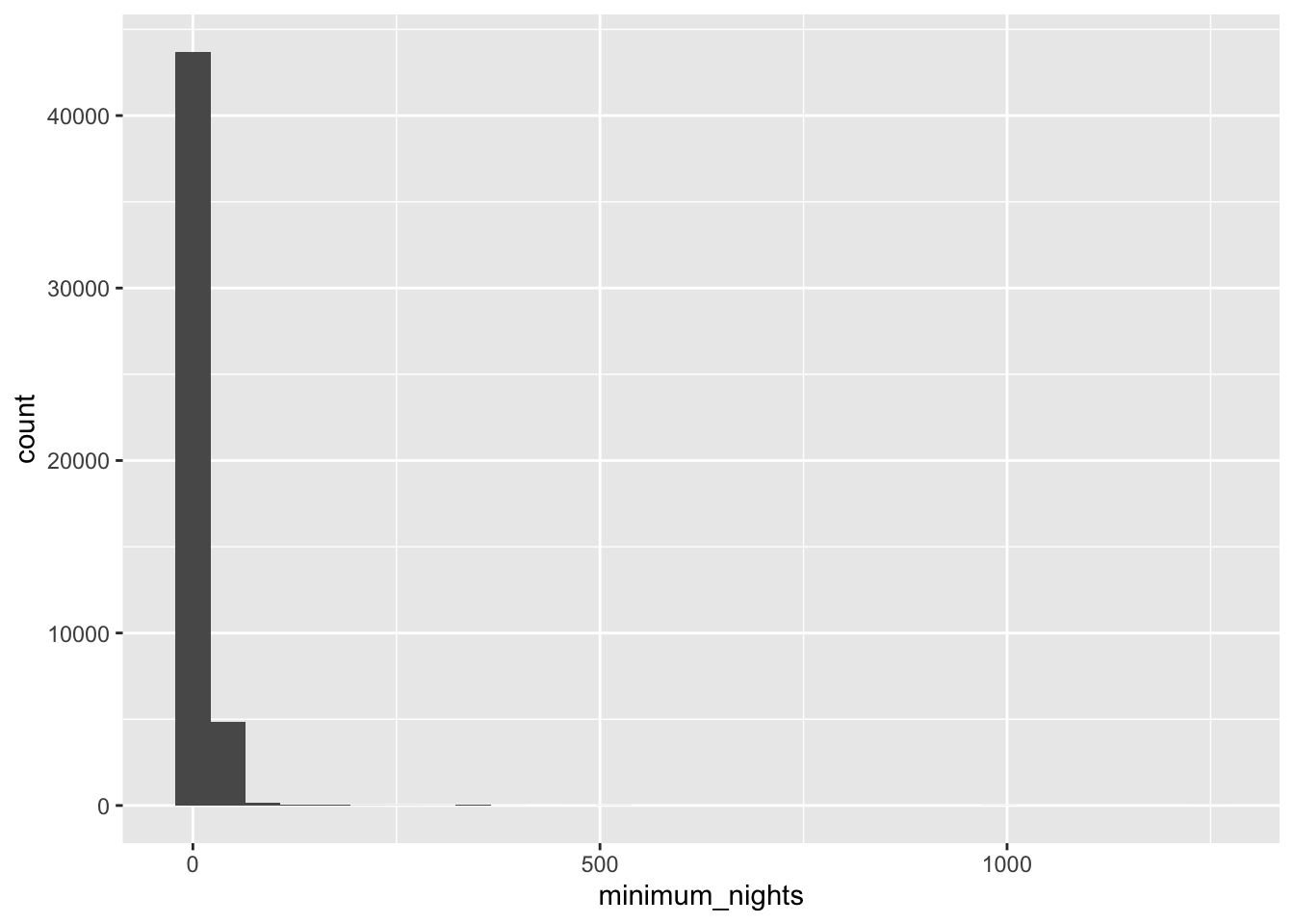
For minimum_nights varible, the plotted histograms presents outliers, let’s remove them.
less_than_400 = airb%>%
  filter(minimum_nights < 400)
ggplot(less_than_400,aes(minimum_nights))+
  geom_histogram()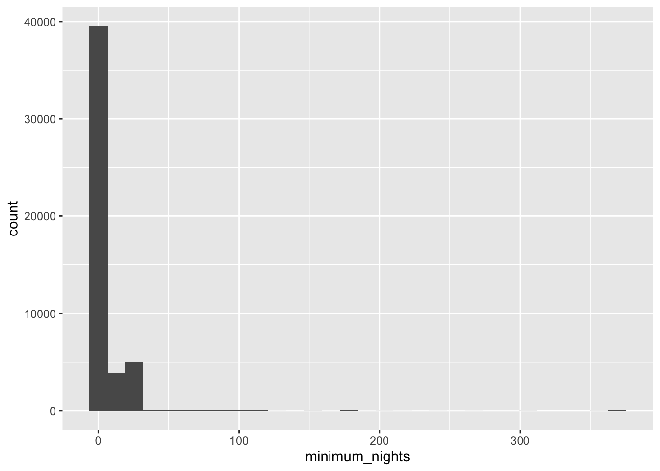
For minimum_nights varible, the plotted histograms presents outliers, let’s remove them.
less_than_200 = airb%>%
  filter(minimum_nights < 200)
ggplot(less_than_200,aes(minimum_nights))+
  geom_histogram()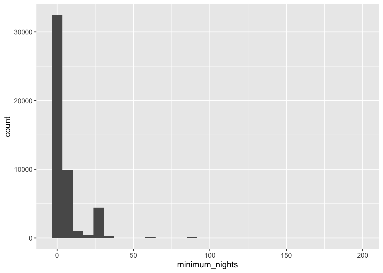
Clearly we have more outliers, let’s filter data even more.
less_than_40 <- airb%>%
  filter(minimum_nights < 40)
ggplot(less_than_40,aes(minimum_nights))+
  geom_histogram()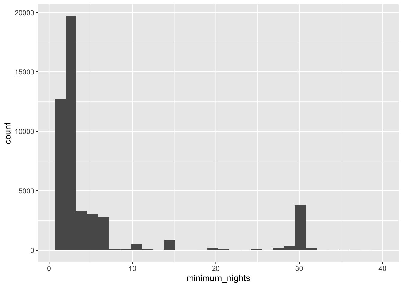
The shape has two humps. It is bimobal.
Visualization with Multiple Dimensions
Now let’s consider rooms types and how they relate to the minimmum nights.
less_than_40 %>%
  ggplot(aes(room_type,minimum_nights))+
  geom_boxplot(alpha=.6)+
  scale_y_continuous(labels=scales::number_format())+
  labs(x="Type of room",
       y="number of nigths")+
  ggthemes::theme_few()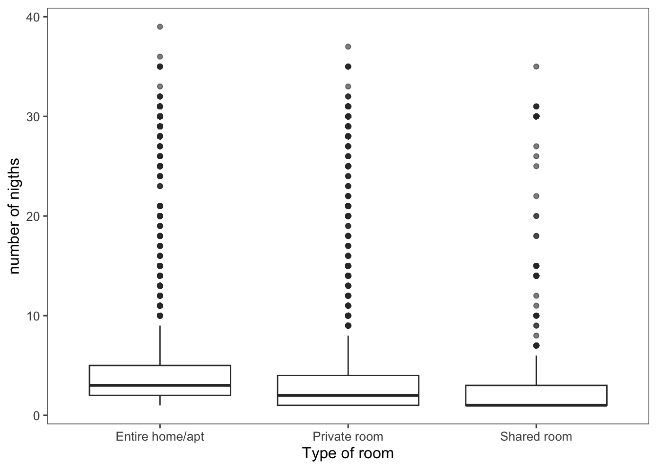
Now, lets check the minimmum nights per neighbourhood group and check if follow the same bimodal distribution.
less_than_40 %>%
  ggplot(aes(minimum_nights))+
  geom_histogram()+
  facet_wrap(vars(neighbourhood_group),scales="free")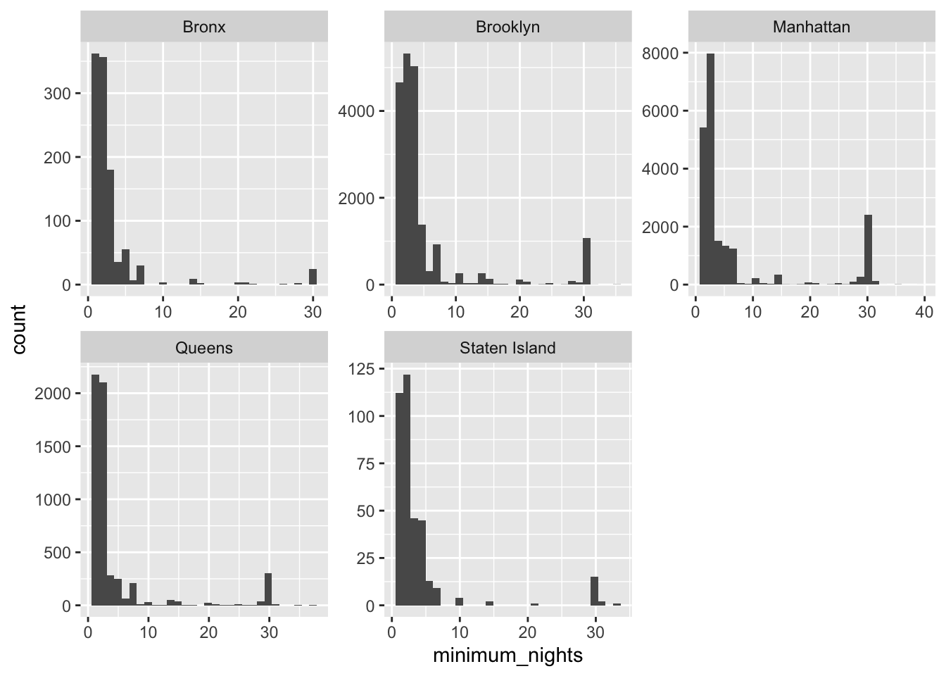
We can observe that all the neighbourhoods follow the same distribution. This suggests they have the same behavior when in terms of minimum nights.
Now, let’s create a new column that shows 5-day intervals for minimum nights. Because there are outliers we take values below 200 minimum nights. We filtered this data in previous steps.
nights_ranges_by_5_days <- less_than_200 %>%
  mutate(nights_ranges = case_when(
    minimum_nights <= 5  ~ "1_5",
    minimum_nights > 5  & minimum_nights <= 10  ~ "5-10",
    minimum_nights > 10  & minimum_nights <= 15  ~ "10-15",
    minimum_nights > 15  & minimum_nights <= 20  ~ "15-20",
    minimum_nights > 20  & minimum_nights <= 25  ~ "20-25",
    minimum_nights > 25  & minimum_nights <= 30  ~ "25-30",
    minimum_nights > 30  & minimum_nights <= 35  ~ "30-35",
    minimum_nights > 35  & minimum_nights <= 40  ~ "35-40",
    minimum_nights > 40  & minimum_nights <= 45  ~ "40-45",
    minimum_nights > 45  & minimum_nights <= 50  ~ "45-50",
    minimum_nights > 50  & minimum_nights <= 55  ~ "50-55",
    minimum_nights > 55  & minimum_nights <= 100  ~ "55-100",
    minimum_nights > 100 ~ "+100" ))%>%
  fill(nights_ranges, .direction = "down")

nights_ranges_by_5_days_factor <- nights_ranges_by_5_days %>%
  mutate( nights_ranges = factor(nights_ranges))
Let’s check the intervals were created.
summary(nights_ranges_by_5_days_factor) id name host_id host_name
Min. : 2539 Length:48822 Min. : 2438 Length:48822
1st Qu.: 9476788 Class :character 1st Qu.: 7831209 Class :character
Median :19692584 Mode :character Median : 30844240 Mode :character
Mean :19025154 Mean : 67666153
3rd Qu.:29156076 3rd Qu.:107434423
Max. :36487245 Max. :274321313
neighbourhood_group neighbourhood latitude longitude
Length:48822 Length:48822 Min. :40.50 Min. :-74.24
Class :character Class :character 1st Qu.:40.69 1st Qu.:-73.98
Mode :character Mode :character Median :40.72 Median :-73.96
Mean :40.73 Mean :-73.95
3rd Qu.:40.76 3rd Qu.:-73.94
Max. :40.91 Max. :-73.71
room_type price minimum_nights number_of_reviews
Length:48822 Min. : 0.0 Min. : 1.000 Min. : 0.00
Class :character 1st Qu.: 69.0 1st Qu.: 1.000 1st Qu.: 1.00
Mode :character Median : 105.5 Median : 2.000 Median : 5.00
Mean : 152.6 Mean : 6.461 Mean : 23.29
3rd Qu.: 175.0 3rd Qu.: 5.000 3rd Qu.: 24.00
Max. :10000.0 Max. :198.000 Max. :629.00
last_review reviews_per_month calculated_host_listings_count
Min. :2011-03-28 Min. : 0.010 Min. : 1.000
1st Qu.:2018-07-10 1st Qu.: 0.190 1st Qu.: 1.000
Median :2019-05-19 Median : 0.720 Median : 1.000
Mean :2018-10-04 Mean : 1.374 Mean : 7.152
3rd Qu.:2019-06-23 3rd Qu.: 2.020 3rd Qu.: 2.000
Max. :2019-07-08 Max. :58.500 Max. :327.000
NA's :10020 NA's :10020
availability_365 nights_ranges
Min. : 0.0 1_5 :38752
1st Qu.: 0.0 25-30 : 4336
Median : 45.0 5-10 : 3503
Mean :112.6 10-15 : 1019
3rd Qu.:226.0 15-20 : 291
Max. :365.0 55-100 : 273
(Other): 648 Now, let see the 5-day intervals for minimum nights and how they relate to the average price for each interval.
nights_ranges_by_5_days_factor %>%

  group_by(nights_ranges) %>%
  summarise(mean_price=mean(price)) %>%
  ggplot(aes(reorder(nights_ranges,-mean_price), mean_price))+
  geom_col()+
  labs(x="minimum_nights ranges in days")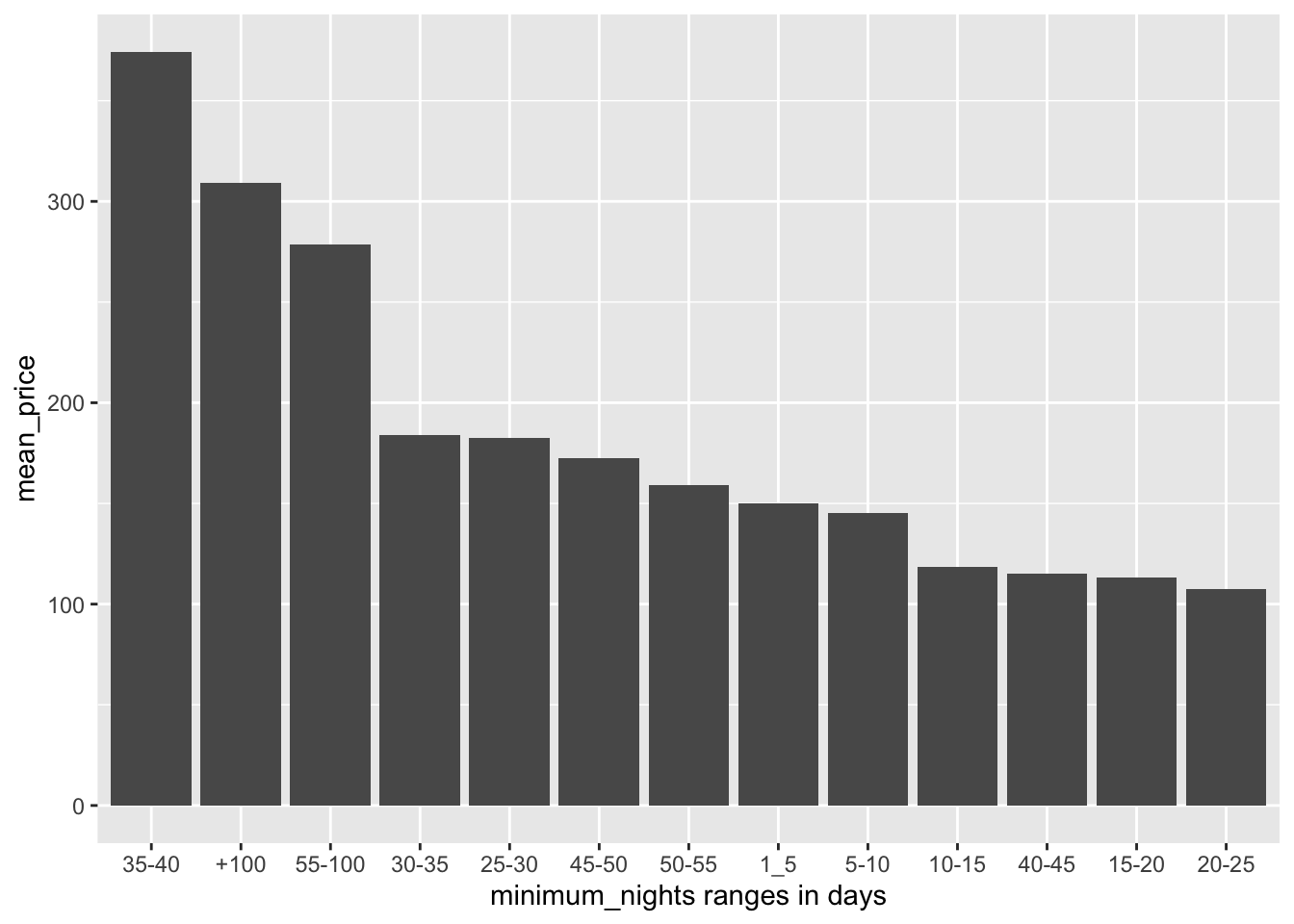
After tailoring the outliers, minimum_nights less than 200, data suggests that for minimum nights between 35 and 40, a host might charge around 365 dollars in average which is higer than minimum nights between 1 and 5, where the host might charge 150 dollars dollars in average.
However, if the 1-5-day hosts were able to rent the at least 4 consecutive times (4 _ 20 days), then the income would be higher in average compared to the 35-40-day hosts.
From the host perspective, data suggest that it is more profitable to rent a house for less number of days compared to other minimum nights 5-day interval.