library(tidyverse)
library(ggplot2)

knitr::opts_chunk$set(echo = TRUE, warning=FALSE, message=FALSE)
Challenge 8
challenge_8
maanusri balasubramanian
snl
Joining Data
Challenge Overview
Today’s challenge is to:
- read in multiple data sets, and describe the data set using both words and any supporting information (e.g., tables, etc)
- tidy data (as needed, including sanity checks)
- mutate variables as needed (including sanity checks)
- join two or more data sets and analyze some aspect of the joined data
(be sure to only include the category tags for the data you use!)
Read in data
Read in one (or more) of the following datasets, using the correct R package and command.
- military marriages ⭐⭐
- faostat ⭐⭐
- railroads ⭐⭐⭐
- fed_rate ⭐⭐⭐
- debt ⭐⭐⭐
- us_hh ⭐⭐⭐⭐
- snl ⭐⭐⭐⭐⭐
# reading the datasets from CSV
snl_actors <- read.csv("_data/snl_actors.csv")
snl_casts <- read.csv("_data/snl_casts.csv")
snl_seasons <- read.csv("_data/snl_seasons.csv")

# peaking into the datasets
head(snl_actors)
aid url type gender
1 Kate McKinnon /Cast/?KaMc cast female
2 Alex Moffat /Cast/?AlMo cast male
3 Ego Nwodim /Cast/?EgNw cast unknown
4 Chris Redd /Cast/?ChRe cast male
5 Kenan Thompson /Cast/?KeTh cast male
6 Carey Mulligan /Guests/?3677 guest andyhead(snl_casts) aid sid featured first_epid last_epid update_anchor n_episodes
1 A. Whitney Brown 11 True 19860222 NA False 8
2 A. Whitney Brown 12 True NA NA False 20
3 A. Whitney Brown 13 True NA NA False 13
4 A. Whitney Brown 14 True NA NA False 20
5 A. Whitney Brown 15 True NA NA False 20
6 A. Whitney Brown 16 True NA NA False 20
season_fraction
1 0.4444444
2 1.0000000
3 1.0000000
4 1.0000000
5 1.0000000
6 1.0000000head(snl_seasons) sid year first_epid last_epid n_episodes
1 1 1975 19751011 19760731 24
2 2 1976 19760918 19770521 22
3 3 1977 19770924 19780520 20
4 4 1978 19781007 19790526 20
5 5 1979 19791013 19800524 20
6 6 1980 19801115 19810411 13# number of rows in each
nrow(snl_actors)[1] 2306nrow(snl_casts)[1] 614nrow(snl_seasons)[1] 46# number of columns in each
ncol(snl_actors)[1] 4ncol(snl_casts)[1] 8ncol(snl_seasons)[1] 5# print column names of each
colnames(snl_actors)[1] "aid" "url" "type" "gender"colnames(snl_casts)[1] "aid" "sid" "featured" "first_epid"
[5] "last_epid" "update_anchor" "n_episodes" "season_fraction"colnames(snl_seasons)[1] "sid" "year" "first_epid" "last_epid" "n_episodes"Briefly describe the data
These 3 datasets contain data about Saturday Night Live actors, casts and seasons respectively. Based on the number of rows, number of columns and column names information from above, we know that there were a total of 2306 actors and 46 seasons in Saturday Night Live. snl_actors dataset contains specific information about actors, snl_casts dataset contains information about the appearance of the show cast (like if they were featured in the show, their episode of appearance, number of episodes of appearance, etc.) and the snl_seasons dataset contains information about each season of the show (like the start episode, the end episode, year it was aired and the number of episodes in the season)
Tidy Data (as needed)
Is your data already tidy, or is there work to be done? Be sure to anticipate your end result to provide a sanity check, and document your work here.
The data is already tidy, so no extra work needs to be done.
Are there any variables that require mutation to be usable in your analysis stream? For example, do you need to calculate new values in order to graph them? Can string values be represented numerically? Do you need to turn any variables into factors and reorder for ease of graphics and visualization?
Document your work here.
Join Data
Be sure to include a sanity check, and double-check that case count is correct!
# Merging snl_actors and snl_casts
cast_actor <- merge(snl_casts, snl_actors, by = 'aid')

# merging cast_actor and snl_seasons
cast_actor_season <- cast_actor %>%
  merge(snl_seasons, by = 'sid') %>%
  group_by(sid, year, gender) %>%
  count(sid, gender)

# plotting gender count over the years
cast_actor_season %>%
  ggplot(aes(year, n, col = gender)) +
  geom_line() +
  ylab("Count") +
  ggtitle("Gender count by year")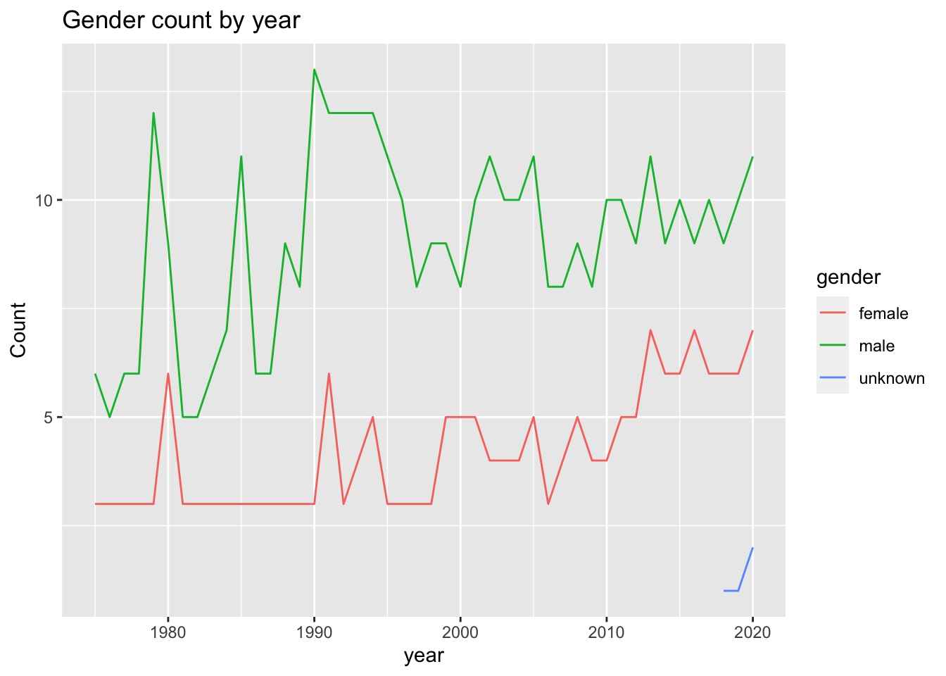
cast_actor_season # A tibble: 95 × 4
# Groups: sid, year, gender [95]
sid year gender n
<int> <int> <chr> <int>
1 1 1975 female 3
2 1 1975 male 6
3 2 1976 female 3
4 2 1976 male 5
5 3 1977 female 3
6 3 1977 male 6
7 4 1978 female 3
8 4 1978 male 6
9 5 1979 female 3
10 5 1979 male 12
# ℹ 85 more rowsFrom the above visualization we can see that there is rise in number of employees in each season over the years.
We can see that there is an increase in the number of actors in the show over the years, which is expected. The number of female actors is lesser than the number of male actors over the years too. We can also see that characters are being added and removed from the show on a regular basis, so the kinks in the graph.