-- Attaching packages --------------------------------------- tidyverse 1.3.2 --
v ggplot2 3.4.1     v purrr   1.0.1
v tibble  3.1.8     v dplyr   1.1.0
v tidyr   1.3.0     v stringr 1.5.0
v readr   2.1.4     v forcats 1.0.0
-- Conflicts ------------------------------------------ tidyverse_conflicts() --
x dplyr::filter() masks stats::filter()
x dplyr::lag()    masks stats::lag()
In this part, you should introduce the dataset(s) and your research questions.
Dataset(s) Introduction:
The main dataset comes from Partners in Flight, a set of databases published by the Bird Conservancy of the Rockies for tracking the estimated poulations of various bird species across various geographic regions.
In this dataset, a case is a species-state - a particular bird species as it occurs in a particular US state, among land birds in the lower 48 states and Alaska. (The dataset does not include Hawaii or the District of Columbia. It does include Canadian provinces and territories, though I will keep the focus of my analysis to the United States.)
The dataset provides several different population estimates for each species-state (main, upper and lower 80% and 95% bounds, median estimate, and unrounded estimate); I will use the main estimate that is simply titled Population Estimate.
Citation for main dataset: Partners in Flight. 2020. Population Estimates Database, version 3.1. Available at http://pif.birdconservancy.org/PopEstimates. Accessed on April 9, 2023.
Citation for dataset used for state population densities: “United States by Density 2020.” n.d. Worldpopulationreview.com. https://worldpopulationreview.com/state-rankings/state-densities.
What questions do you like to answer with this dataset(s)?
I will use this dataset to compute the population density of bird species in the United States by state and compare it with states’ human population densities, to answer the question of which bird species are associated positively with human population density and which negatively so. Although this would not in and of itself prove that development causes harm to bird populations, it could shed light on which bird species might benefit from further research to determine if they are being adversely affected by development in areas with dense human populations.
tibble [8,805 x 28] (S3: tbl_df/tbl/data.frame)
 $ Sequence AOS 60                     : num [1:8805] 83 96 96 96 96 101 101 101 101 101 ...
 $ English Name                        : chr [1:8805] "Plain Chachalaca" "Mountain Quail" "Mountain Quail" "Mountain Quail" ...
 $ Scientific Name                     : chr [1:8805] "Ortalis vetula" "Oreortyx pictus" "Oreortyx pictus" "Oreortyx pictus" ...
 $ Introduced                          : chr [1:8805] NA NA NA NA ...
 $ Province / State / Territory        : chr [1:8805] "TX" "CA" "OR" "NV" ...
 $ Country                             : chr [1:8805] "USA" "USA" "USA" "USA" ...
 $ Population Estimate                 : num [1:8805] NA 230000 25000 910 170 NA NA NA NA NA ...
 $ Lower 95% bound                     : num [1:8805] NA 150000 13000 490 0 NA NA NA NA NA ...
 $ Upper 95% bound                     : num [1:8805] NA 320000 41000 1600 840 NA NA NA NA NA ...
 $ Data Source                         : chr [1:8805] NA "bbs" "bbs" "bbs,rng" ...
 $ Estimated % of Global Population    : num [1:8805] NA 0.877845 0.095676 0.003541 0.000646 ...
 $ Estimated % of USA/Canada Population: num [1:8805] NA 0.897861 0.097857 0.003622 0.000661 ...
 $ Median Estimate                     : num [1:8805] NA 220000 23000 860 67 NA NA NA NA NA ...
 $ Lower 80% bound                     : num [1:8805] NA 170000 16000 590 0 NA NA NA NA NA ...
 $ Upper 80% bound                     : num [1:8805] NA 290000 35000 1300 470 NA NA NA NA NA ...
 $ BBS Average (birds/rte)             : num [1:8805] 0.00489 2.22934 0.39827 0.01288 0.00382 ...
 $ BBS Routes                          : num [1:8805] 204 191 99 30 85 204 61 53 70 46 ...
 $ Species Routes                      : num [1:8805] 1 104 30 0 1 163 60 53 68 36 ...
 $ Area of Region      (km2)           : num [1:8805] 687020 410207 250255 286367 176218 ...
 $ Detection Distance Category (m)     : num [1:8805] 300 300 300 300 300 200 200 200 200 200 ...
 $ Pair Adjust Category                : num [1:8805] 2 2 2 2 2 1.75 1.75 1.75 1.75 1.75 ...
 $ Time Adjust Mean                    : num [1:8805] 1.65 1.5 1.5 1.5 1.5 ...
 $ Time Adjust             SD          : num [1:8805] 0.2246 0.0217 0.0217 0.0217 0.0217 ...
 $ Population Estimate (unrounded)     : num [1:8805] NA 225206 24545 908 166 ...
 $ Lower 80% bound (unrounded)         : num [1:8805] NA 171416 16058 589 0 ...
 $ Upper 80% bound (unrounded)         : num [1:8805] NA 286830 34774 1296 465 ...
 $ Lower 95% bound (unrounded)         : num [1:8805] NA 150115 13038 487 0 ...
 $ Upper 95% bound (unrounded)         : num [1:8805] NA 322391 40930 1586 843 ...
conduct summary statistics of the dataset(s); especially show the basic statistics (min, max, mean, median, etc.) for the variables you are interested in.
In the PIF bird populations by state dataset, each row represents a bird species as it occurs in a given US state (except Hawaii) or Canadian province/territory. This analysis focuses on US data, so the Canadian data have been dropped. There are 7,030 observations of species-state, with 27 variables about each species-state collected. The variables most relevant to this analysis, which will examine bird species’ population density in each state, are the bird’s English Name, its State, and its Population Estimate. A median population estimate and an unrounded population estimate, as well as upper and lower 80% and 95% population estimates for each species, are also given, although as of now I am likely to stick with basing my analysis on the main Population Estimate for each species.
In the state statistics dataset, each row represents a state. There are 50 observations, with each case being a US state. The various columns include ones representing the state’s name, its population density, its population in 2023 and various recent past years, its population growth rate, and its total land area. For this analysis, I kept only four columns: state name (converted to an abbreviation), population density, 2023 population, and total area.
The overall combined dataset contains 7,030 observations of 30 variables - all of the variables from the birds dataset, and the four variables retained from the state statistics dataset. (Ultimately, there are likely to be fewer variables as I drop some of the less relevant variables from the birds dataset). Additionally, I will use the information in the Population Estimate and TotalArea columns to create a new column containing the population density of each bird species in each state.
Note: Changes made since Assignment 1 submission
-Reading in the forest and water area data -Replacing NAs with zeroes -+
3. The Plan for Visualization
Briefly describe what data analyses (please the special note on statistics in the next section) and visualizations you plan to conduct to answer the research questions you proposed above.
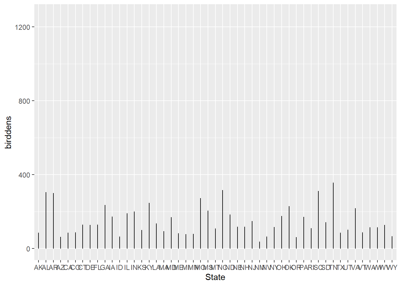
I plan to divide the Population Estimate column by the TotalArea column to compute the population density for each bird species in each state. Then, I will create a line graph for each species with state on the horizontal axis and population density on the vertical axis; with human population density as another line for easy comparison on the same graph.
I will also graph population density of species against the states’ percent forest area and percent water area.
Explain why you choose to conduct these specific data analyses and visualizations. In other words, how do such types of statistics or graphs (see the R Gallery) help you answer specific questions? For example, how can a bivariate visualization reveal the relationship between two variables, or how does a linear graph of variables over time present the pattern of development?
Graphing bird species’ population densities in each state against human population density in the same state will let it be readily seen how the population density of each species is related to that of humanity, state by state. Although it can’t prove causality, it can provide some evidence of which species are thriving in areas highly settled by humanity and which are suffering in similar areas.
If you plan to conduct specific data analyses and visualizations, describe how do you need to process and prepare the tidy data.
What do you need to do to mutate the datasets (convert date data, create a new variable, pivot the data format, etc.)?
The main necessities are to decide on an approach for handling NA values of population for certain species-states and to calculate the new column of species population densities.
- How are you going to deal with the missing data/NAs and outliers? And why do you choose this way to deal with NAs?
I have replaced my NAs in species-state cases with zeroes. There are only 38 species with completely missing Population Estimates (out of 404 in the database), and most of them are either fowl or birds whose populations one would not expect to be large enough to be reliably estimated or to substantially affect the overall analysis (certain birds of prey, endangered species, and predominantly Canadian or Mexican species whose breeding ranges only slightly extend into the United States). There are also some NAs for specific states for species whose breeding ranges extend only very slightly into those states. I will give my results the caveat that they are not applicable to fowl, birds of prey, and waterfowl (which are not included in the dataset in the first place). There is no apparent way to fill in the missing data, at least from sources that would be methodologically consistent with and comparable to the PIF database. Though this approach is not without its downsides, since the low-population species that would be excluded are potentially some of the most relevant for conservation purposes, it makes sense to replace NAs with zeroes because the populations of birds with missing values are likely small enough compared to those of more common birds (many of which count millions of individuals in some states) to be effectively zero.
(Optional) It is encouraged, but optional, to include a coding component of tidy data in this part.
Graphing bird density by vs. human density by state and species:
---title: "Final Project Assignment#2: Matt Eckstein"author: "Matt Eckstein"description: "Matt Eckstein Final Project Assignment 2 - Bird Visualizations"date: "05-02-2023"format: html: df-print: paged toc: true code-copy: true code-tools: true css: styles.csscategories: - final_Project_assignment_1 - final_project_data_descriptioneditor_options: chunk_output_type: console---```{r}#| label: setup#| warning: false#| message: falselibrary(tidyverse)knitr::opts_chunk$set(echo =TRUE, warning=FALSE, message=FALSE)```## Part 1. Introduction {#describe-the-data-sets}In this part, you should introduce the dataset(s) and your research questions.1. Dataset(s) Introduction:The main dataset comes from Partners in Flight, a set of databases published by the Bird Conservancy of the Rockies for tracking the estimated poulations of various bird species across various geographic regions.In this dataset, a case is a species-state - a particular bird species as it occurs in a particular US state, among land birds in the lower 48 states and Alaska. (The dataset does not include Hawaii or the District of Columbia. It does include Canadian provinces and territories, though I will keep the focus of my analysis to the United States.)The dataset provides several different population estimates for each species-state (main, upper and lower 80% and 95% bounds, median estimate, and unrounded estimate); I will use the main estimate that is simply titled Population Estimate.Citation for main dataset: Partners in Flight. 2020. Population Estimates Database, version 3.1. Available at http://pif.birdconservancy.org/PopEstimates. Accessed on April 9, 2023.Citation for dataset used for state population densities: "United States by Density 2020." n.d. Worldpopulationreview.com. https://worldpopulationreview.com/state-rankings/state-densities.2. What questions do you like to answer with this dataset(s)?I will use this dataset to compute the population density of bird species in the United States by state and compare it with states' human population densities, to answer the question of which bird species are associated positively with human population density and which negatively so. Although this would not in and of itself prove that development causes harm to bird populations, it could shed light on which bird species might benefit from further research to determine if they are being adversely affected by development in areas with dense human populations.## Part 2. Describe the data set(s) {#describe-the-data-sets-1}```{r}library(readxl)birds <-read_xlsx("MattEckstein_FinalProjectData/PopEsts_ProvState_2021.02.05.xlsx")str(birds)#renaming State variable for compatibility with the state population density dataset birds <-rename(birds, "State"="Province / State / Territory")#dropping if the country is Canada, then removing the country variablebirds <-select(birds, -c(`Sequence AOS 60`, `Data Source`, `Pair Adjust Category`, `Introduced`, `Estimated % of Global Population`, `Estimated % of USA/Canada Population`, `BBS Average (birds/rte)`, `BBS Routes`, `Species Routes`, `Detection Distance Category (m)`, `Pair Adjust Category`, `Time Adjust Mean`, `Time Adjust SD`))birds <-subset(birds, Country !="CAN")birds <-select(birds, -c(Country))states <-read_csv("MattEckstein_FinalProjectData/State_statistics.csv")#dropping variables that are unlikely to be useful for analysis, for the sake of neatnessstates <-select(states, -c(pop2022, pop2020, pop2019, pop2010, growthRate, growth, growthSince2010, fips))#replacing state names with abbreviations, for compatibility among the starting datasetsstates[states =='New Jersey'] <-'NJ'states[states =='Rhode Island'] <-'RI'states[states =='Massachusetts'] <-'MA'states[states =='Connecticut'] <-'CT'states[states =='Maryland'] <-'MD'states[states =='Delaware'] <-'DE'states[states =='Florida'] <-'FL'states[states =='New York'] <-'NY'states[states =='Pennsylvania'] <-'PA'states[states =='Ohio'] <-'OH'states[states =='California'] <-'CA'states[states =='Illinois'] <-'IL'states[states =='Hawaii'] <-'HI'states[states =='North Carolina'] <-'NC'states[states =='Virginia'] <-'VA'states[states =='Georgia'] <-'GA'states[states =='Indiana'] <-'IN'states[states =='South Carolina'] <-'SC'states[states =='Michigan'] <-'MI'states[states =='Tennessee'] <-'TN'states[states =='New Hampshire'] <-'NH'states[states =='Washington'] <-'WA'states[states =='Texas'] <-'TX'states[states =='Kentucky'] <-'KY'states[states =='Wisconsin'] <-'WI'states[states =='Louisiana'] <-'LA'states[states =='Alabama'] <-'AL'states[states =='Missouri'] <-'MO'states[states =='West Virginia'] <-'WV'states[states =='Minnesota'] <-'MN'states[states =='Vermont'] <-'VT'states[states =='Arizona'] <-'AZ'states[states =='Mississippi'] <-'MS'states[states =='Oklahoma'] <-'OK'states[states =='Arkansas'] <-'AR'states[states =='Iowa'] <-'IA'states[states =='Colorado'] <-'CO'states[states =='Maine'] <-'ME'states[states =='Oregon'] <-'OR'states[states =='Utah'] <-'UT'states[states =='Kansas'] <-'KS'states[states =='Nevada'] <-'NV'states[states =='Nebraska'] <-'NE'states[states =='Idaho'] <-'ID'states[states =='New Mexico'] <-'NM'states[states =='South Dakota'] <-'SD'states[states =='North Dakota'] <-'ND'states[states =='Montana'] <-'MT'states[states =='Wyoming'] <-'WY'states[states =='Alaska'] <-'AK'forest <-read_csv("MattEckstein_FinalProjectData/State_forests.csv")#dropping variables that are unlikely to be useful for analysis, for the sake of neatnessforest <-select(forest, -c(pop2023, pop2022, pop2020, pop2019, pop2010, growthRate, growth, growthSince2010, fips, rank, densityMi))#replacing state names with abbreviations, for compatibility among the starting datasetsforest[forest =='New Jersey'] <-'NJ'forest[forest =='Rhode Island'] <-'RI'forest[forest =='Massachusetts'] <-'MA'forest[forest =='Connecticut'] <-'CT'forest[forest =='Maryland'] <-'MD'forest[forest =='Delaware'] <-'DE'forest[forest =='Florida'] <-'FL'forest[forest =='New York'] <-'NY'forest[forest =='Pennsylvania'] <-'PA'forest[forest =='Ohio'] <-'OH'forest[forest =='California'] <-'CA'forest[forest =='Illinois'] <-'IL'forest[forest =='Hawaii'] <-'HI'forest[forest =='North Carolina'] <-'NC'forest[forest =='Virginia'] <-'VA'forest[forest =='Georgia'] <-'GA'forest[forest =='Indiana'] <-'IN'forest[forest =='South Carolina'] <-'SC'forest[forest =='Michigan'] <-'MI'forest[forest =='Tennessee'] <-'TN'forest[forest =='New Hampshire'] <-'NH'forest[forest =='Washington'] <-'WA'forest[forest =='Texas'] <-'TX'forest[forest =='Kentucky'] <-'KY'forest[forest =='Wisconsin'] <-'WI'forest[forest =='Louisiana'] <-'LA'forest[forest =='Alabama'] <-'AL'forest[forest =='Missouri'] <-'MO'forest[forest =='West Virginia'] <-'WV'forest[forest =='Minnesota'] <-'MN'forest[forest =='Vermont'] <-'VT'forest[forest =='Arizona'] <-'AZ'forest[forest =='Mississippi'] <-'MS'forest[forest =='Oklahoma'] <-'OK'forest[forest =='Arkansas'] <-'AR'forest[forest =='Iowa'] <-'IA'forest[forest =='Colorado'] <-'CO'forest[forest =='Maine'] <-'ME'forest[forest =='Oregon'] <-'OR'forest[forest =='Utah'] <-'UT'forest[forest =='Kansas'] <-'KS'forest[forest =='Nevada'] <-'NV'forest[forest =='Nebraska'] <-'NE'forest[forest =='Idaho'] <-'ID'forest[forest =='New Mexico'] <-'NM'forest[forest =='South Dakota'] <-'SD'forest[forest =='North Dakota'] <-'ND'forest[forest =='Montana'] <-'MT'forest[forest =='Wyoming'] <-'WY'forest[forest =='Alaska'] <-'AK'area <-read_csv("MattEckstein_FinalProjectData/State_waterarea.csv")area <-select(area, -c(densityMi, TotalArea, pop2023, pop2022, pop2020, pop2019, pop2010, growthRate, growth, growthSince2010, fips, rank))area[area =='New Jersey'] <-'NJ'area[area =='Rhode Island'] <-'RI'area[area =='Massachusetts'] <-'MA'area[area =='Connecticut'] <-'CT'area[area =='Maryland'] <-'MD'area[area =='Delaware'] <-'DE'area[area =='Florida'] <-'FL'area[area =='New York'] <-'NY'area[area =='Pennsylvania'] <-'PA'area[area =='Ohio'] <-'OH'area[area =='California'] <-'CA'area[area =='Illinois'] <-'IL'area[area =='Hawaii'] <-'HI'area[area =='North Carolina'] <-'NC'area[area =='Virginia'] <-'VA'area[area =='Georgia'] <-'GA'area[area =='Indiana'] <-'IN'area[area =='South Carolina'] <-'SC'area[area =='Michigan'] <-'MI'area[area =='Tennessee'] <-'TN'area[area =='New Hampshire'] <-'NH'area[area =='Washington'] <-'WA'area[area =='Texas'] <-'TX'area[area =='Kentucky'] <-'KY'area[area =='Wisconsin'] <-'WI'area[area =='Louisiana'] <-'LA'area[area =='Alabama'] <-'AL'area[area =='Missouri'] <-'MO'area[area =='West Virginia'] <-'WV'area[area =='Minnesota'] <-'MN'area[area =='Vermont'] <-'VT'area[area =='Arizona'] <-'AZ'area[area =='Mississippi'] <-'MS'area[area =='Oklahoma'] <-'OK'area[area =='Arkansas'] <-'AR'area[area =='Iowa'] <-'IA'area[area =='Colorado'] <-'CO'area[area =='Maine'] <-'ME'area[area =='Oregon'] <-'OR'area[area =='Utah'] <-'UT'area[area =='Kansas'] <-'KS'area[area =='Nevada'] <-'NV'area[area =='Nebraska'] <-'NE'area[area =='Idaho'] <-'ID'area[area =='New Mexico'] <-'NM'area[area =='South Dakota'] <-'SD'area[area =='North Dakota'] <-'ND'area[area =='Montana'] <-'MT'area[area =='Wyoming'] <-'WY'area[area =='Alaska'] <-'AK'#combining datasets into onestates <-rename(states, "State"="state")forest <-rename(forest, "State"="state")area <-rename(area, "State"="state")alldata <-merge(birds, states, by ="State")alldata <-merge(alldata, forest, by ="State")alldata <-merge(alldata, area, by ="State")alldata <-mutate_all(alldata, ~replace_na(.,0))alldata <- alldata %>%mutate(birddens =`Population Estimate`/`TotalArea`)alldata <- alldata %>%mutate(shareforest =`forestArea`/`TotalArea`)alldata <- alldata %>%mutate(sharewater =`WaterArea`/`TotalArea`)alldata <- alldata %>%mutate(pctforest = (`forestArea`/`TotalArea`) *100)alldata <- alldata %>%mutate(pctwater = (`WaterArea`/`TotalArea`) *100)```2. present the descriptive information of the dataset(s) using the functions in Challenges 1, 2, and 3;The overall dataset has 7,030 observations of 31 variables. ```{r}dim(alldata)head(alldata)```3. conduct summary statistics of the dataset(s); especially show the basic statistics (min, max, mean, median, etc.) for the variables you are interested in.```{r}library(vtable)alldata %>% sumtable("Population Estimate")alldata %>% sumtable("Total Area")alldata %>% sumtable("densityMi")```In the PIF bird populations by state dataset, each row represents a bird species as it occurs in a given US state (except Hawaii) or Canadian province/territory. This analysis focuses on US data, so the Canadian data have been dropped. There are 7,030 observations of species-state, with 27 variables about each species-state collected. The variables most relevant to this analysis, which will examine bird species' population density in each state, are the bird's English Name, its State, and its Population Estimate. A median population estimate and an unrounded population estimate, as well as upper and lower 80% and 95% population estimates for each species, are also given, although as of now I am likely to stick with basing my analysis on the main Population Estimate for each species.In the state statistics dataset, each row represents a state. There are 50 observations, with each case being a US state. The various columns include ones representing the state's name, its population density, its population in 2023 and various recent past years, its population growth rate, and its total land area. For this analysis, I kept only four columns: state name (converted to an abbreviation), population density, 2023 population, and total area.The overall combined dataset contains 7,030 observations of 30 variables - all of the variables from the birds dataset, and the four variables retained from the state statistics dataset. (Ultimately, there are likely to be fewer variables as I drop some of the less relevant variables from the birds dataset). Additionally, I will use the information in the Population Estimate and TotalArea columns to create a new column containing the population density of each bird species in each state.## Note: Changes made since Assignment 1 submission-Reading in the forest and water area data-Replacing NAs with zeroes-+ ## 3. The Plan for Visualization {#the-tentative-plan-for-visualization}1. Briefly describe what data analyses (**please the special note on statistics in the next section)** and visualizations you plan to conduct to answer the research questions you proposed above.I plan to divide the Population Estimate column by the TotalArea column to compute the population density for each bird species in each state. Then, I will create a line graph for each species with state on the horizontal axis and population density on the vertical axis; with human population density as another line for easy comparison on the same graph.I will also graph population density of species against the states' percent forest area and percent water area.2. Explain why you choose to conduct these specific data analyses and visualizations. In other words, how do such types of statistics or graphs (see [the R Gallery](https://r-graph-gallery.com/)) help you answer specific questions? For example, how can a bivariate visualization reveal the relationship between two variables, or how does a linear graph of variables over time present the pattern of development?Graphing bird species' population densities in each state against human population density in the same state will let it be readily seen how the population density of each species is related to that of humanity, state by state. Although it can't prove causality, it can provide some evidence of which species are thriving in areas highly settled by humanity and which are suffering in similar areas.3. If you plan to conduct specific data analyses and visualizations, describe how do you need to process and prepare the tidy data. - What do you need to do to mutate the datasets (convert date data, create a new variable, pivot the data format, etc.)?The main necessities are to decide on an approach for handling NA values of population for certain species-states and to calculate the new column of species population densities. - How are you going to deal with the missing data/NAs and outliers? And why do you choose this way to deal with NAs?I have replaced my NAs in species-state cases with zeroes. There are only 38 species with completely missing Population Estimates (out of 404 in the database), and most of them are either fowl or birds whose populations one would not expect to be large enough to be reliably estimated or to substantially affect the overall analysis (certain birds of prey, endangered species, and predominantly Canadian or Mexican species whose breeding ranges only slightly extend into the United States). There are also some NAs for specific states for species whose breeding ranges extend only very slightly into those states. I will give my results the caveat that they are not applicable to fowl, birds of prey, and waterfowl (which are not included in the dataset in the first place). There is no apparent way to fill in the missing data, at least from sources that would be methodologically consistent with and comparable to the PIF database. Though this approach is not without its downsides, since the low-population species that would be excluded are potentially some of the most relevant for conservation purposes, it makes sense to replace NAs with zeroes because the populations of birds with missing values are likely small enough compared to those of more common birds (many of which count millions of individuals in some states) to be effectively zero.4. (Optional) It is encouraged, **but optional**, to include a coding component of tidy data in this part.Graphing bird density by vs. human density by state and species:```{r}#Methodological inspiration from: https://stackoverflow.com/questions/34959213/ggplot2-how-do-i-add-a-second-plot-lineggplot(alldata, aes(x=State)) +geom_line(aes(y=birddens)) +geom_line(aes(y=densityMi)) +facet_wrap(~`English Name`)```Graphing bird density by vs. human density by state:```{r}#Methodological inspiration from: https://stackoverflow.com/questions/34959213/ggplot2-how-do-i-add-a-second-plot-lineggplot(alldata, aes(x=State)) +geom_line(aes(y=birddens)) +geom_line(aes(y=densityMi)) ```Graphing bird density by vs. forest area coverage by state:```{r}ggplot(alldata, aes(x=State)) +geom_line(aes(y=pctforest)) +geom_line(aes(y=densityMi)) ```Graphing bird density by vs. water area coverage by state:```{r}ggplot(alldata, aes(x=State)) +geom_line(aes(y=pctwater)) +geom_line(aes(y=densityMi))```