Challenge 5

cereal

Introduction to Visualization

Author

Matt Eckstein

Published

March 29, 2023

library(tidyverse)
library(ggplot2)

knitr::opts_chunk$set(echo = TRUE, warning=FALSE, message=FALSE)

Read in data

Read in one (or more) of the following datasets, using the correct R package and command.

cereal <- read_csv("_data/cereal.csv")
str(cereal)

spc_tbl_ [20 x 4] (S3: spec_tbl_df/tbl_df/tbl/data.frame)
 $ Cereal: chr [1:20] "Frosted Mini Wheats" "Raisin Bran" "All Bran" "Apple Jacks" ...
 $ Sodium: num [1:20] 0 340 70 140 200 180 210 150 100 130 ...
 $ Sugar : num [1:20] 11 18 5 14 12 1 10 16 0 12 ...
 $ Type  : chr [1:20] "A" "A" "A" "C" ...
 - attr(*, "spec")=
  .. cols(
  ..   Cereal = col_character(),
  ..   Sodium = col_double(),
  ..   Sugar = col_double(),
  ..   Type = col_character()
  .. )
 - attr(*, "problems")=<externalptr>

Briefly describe the data

This dataset lists several popular breakfast cereals by their sodium content, their sugar content, and their type A or C (presumably meaning adult or children’s).

Tidy Data (as needed)

Is your data already tidy, or is there work to be done? Be sure to anticipate your end result to provide a sanity check, and document your work here.

This dataset is already tidy as it is.

#Nothing needed here

Are there any variables that require mutation to be usable in your analysis stream? For example, do you need to calculate new values in order to graph them? Can string values be represented numerically? Do you need to turn any variables into factors and reorder for ease of graphics and visualization?

I have converted the Type variable into a numeric variable.

#Converting types A and C to numeric values 1 and 2
cereal <- cereal%>%
  mutate(Type = case_when(
    Type == "A" ~ 1,
    Type == "C" ~ 2)
         )

#Checking that the variable type was successfully converted
str(cereal)

tibble [20 x 4] (S3: tbl_df/tbl/data.frame)
 $ Cereal: chr [1:20] "Frosted Mini Wheats" "Raisin Bran" "All Bran" "Apple Jacks" ...
 $ Sodium: num [1:20] 0 340 70 140 200 180 210 150 100 130 ...
 $ Sugar : num [1:20] 11 18 5 14 12 1 10 16 0 12 ...
 $ Type  : num [1:20] 1 1 1 2 2 2 2 1 1 2 ...

Univariate Visualizations

I chose to visualize sodium and sugar with histograms because these do a good job of illustrating the distribution of cereals by the amount of each substance they contain. I chose to have 10 bins in each graph because this number provides relatively neat graphs that illustrate that the amount of sodium in cereals clusters around a value just shy of 200 units, while the distribution of the amount of sugar in cereals is relatively uniform

summary(cereal)

    Cereal              Sodium          Sugar            Type    
 Length:20          Min.   :  0.0   Min.   : 0.00   Min.   :1.0  
 Class :character   1st Qu.:137.5   1st Qu.: 4.00   1st Qu.:1.0  
 Mode  :character   Median :180.0   Median : 9.50   Median :1.5  
                    Mean   :167.0   Mean   : 8.75   Mean   :1.5  
                    3rd Qu.:202.5   3rd Qu.:12.50   3rd Qu.:2.0  
                    Max.   :340.0   Max.   :18.00   Max.   :2.0

ggplot(cereal, aes(Sugar)) + geom_histogram(bins = 10)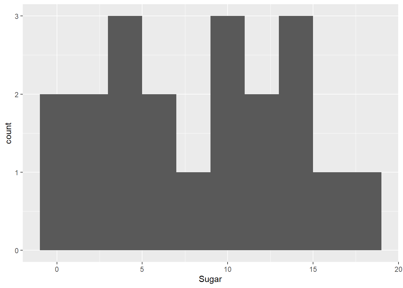

ggplot(cereal, aes(Sodium)) + geom_histogram(bins = 10)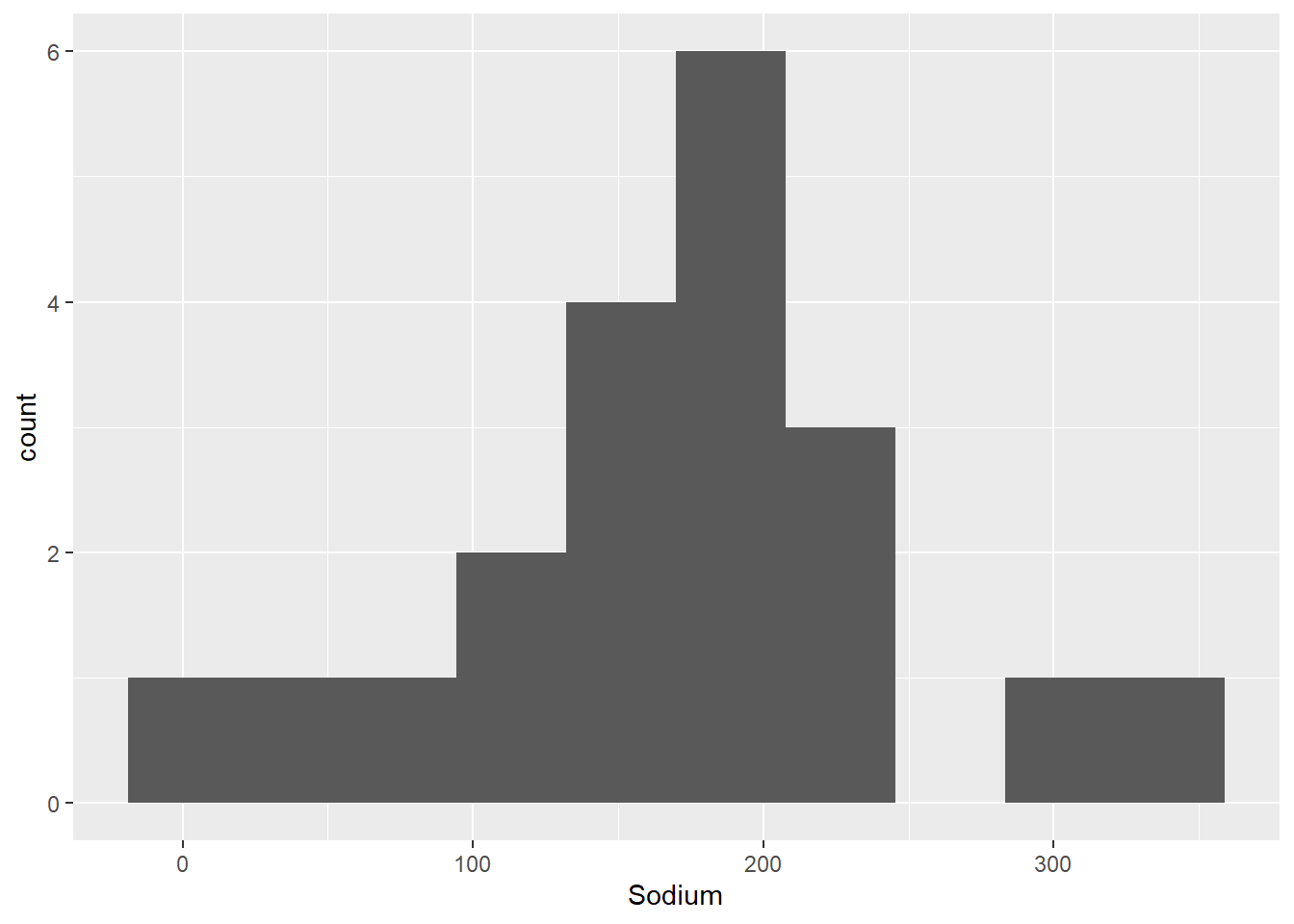

Bivariate Visualization(s)

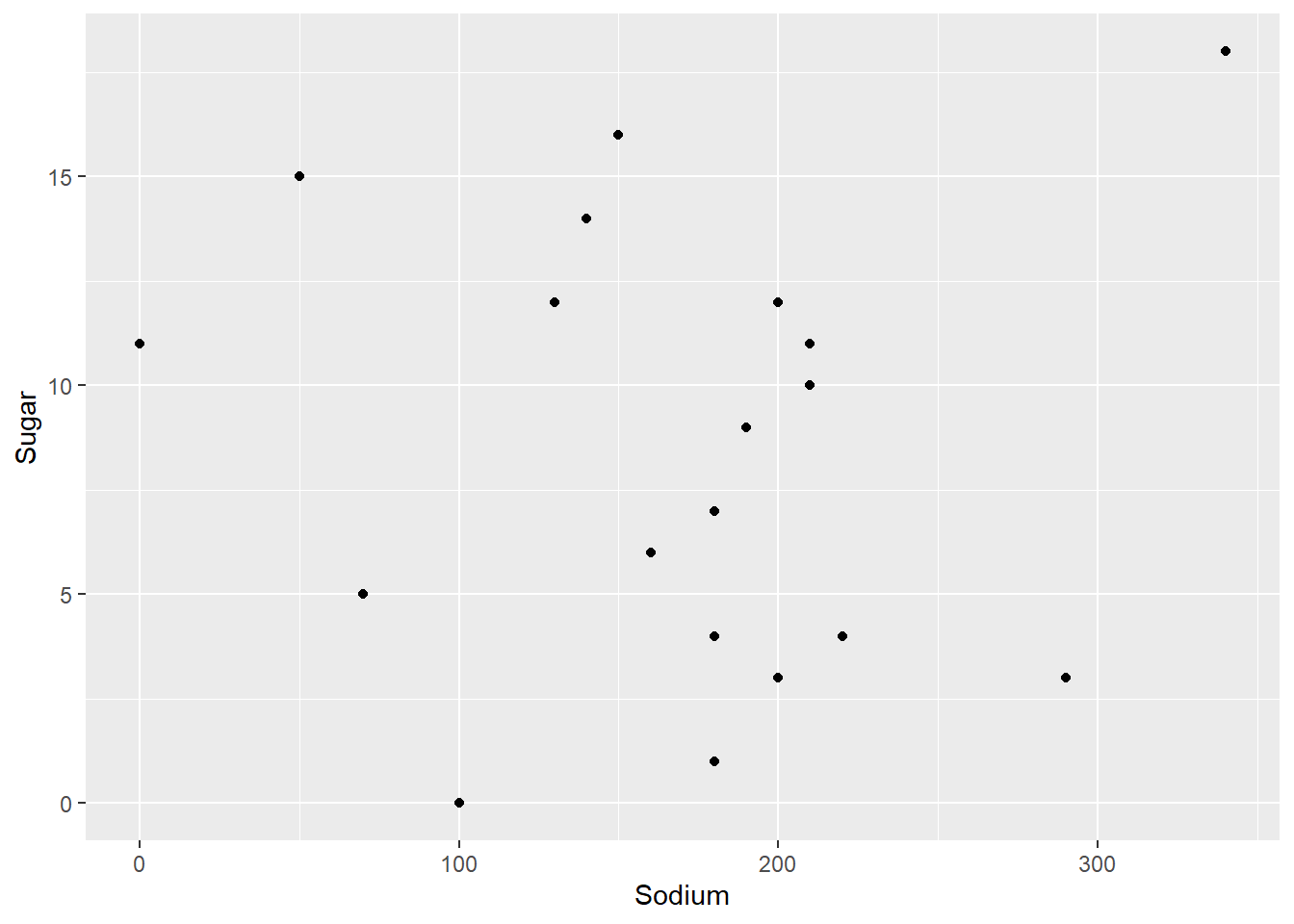
I chose to make a scatterplot in order to see any relationship between the amount of sodium in a cereal and the amount of sugar in one - there is no apparent strong relationship, it turns out.

ggplot(cereal, aes(Sodium, Sugar)) + geom_point()