library(tidyverse)
library(ggplot2)

knitr::opts_chunk$set(echo = TRUE, warning=FALSE, message=FALSE)Challenge 5
challenge_5
cereal
Matthew_Weiner
Introduction to Visualization
Introduction
For this challenge I will be using the cereal.csv dataset
Getting Started
We first need to load in the necessary libraries and then perform some basic analysis on the dataset.
library(readr)
#read dataset
cereal <- read_csv("_data/cereal.csv")

#number of rows in dataset
nrow(cereal)
[1] 20#number of columnns in dataset
ncol(cereal)[1] 4#name of the columns in the dataset
colnames(cereal)[1] "Cereal" "Sodium" "Sugar" "Type" From this basic investigation into the dataset we can see that there are 4 variables: the cereal name, the sodium and sugar contents of the cereal, and finally some label for each entry called “Type”. While we don’t know what the distinction between the different types is yet. We can see that the dataset includes cereals of type A and C.
table(cereal$Type)
 A  C
10 10
We can also view the summary statistics of the dataset using the summary() command:
summary(cereal[, c("Sodium", "Sugar")]) Sodium Sugar
Min. : 0.0 Min. : 0.00
1st Qu.:137.5 1st Qu.: 4.00
Median :180.0 Median : 9.50
Mean :167.0 Mean : 8.75
3rd Qu.:202.5 3rd Qu.:12.50
Max. :340.0 Max. :18.00 Tidy Data
This dataset does not appear to need any tidying. There are no missing values which we can see below, and there are no values for any variables that are unneccessary and should be removed.
sum(is.na(cereal))[1] 0Univariate Visualizations
One interesting aspect of this dataset to explore would be a distrbituion of the amount of sodium in the cereals. I chose to make the binwidth = 10 as I found the default value, 30, was too large and led to the histogram looking too simple and did not properly display some of the outliers.
ggplot(cereal, aes(x = Sodium)) + geom_histogram(binwidth = 10) + ggtitle("Sodium Content in Cereals")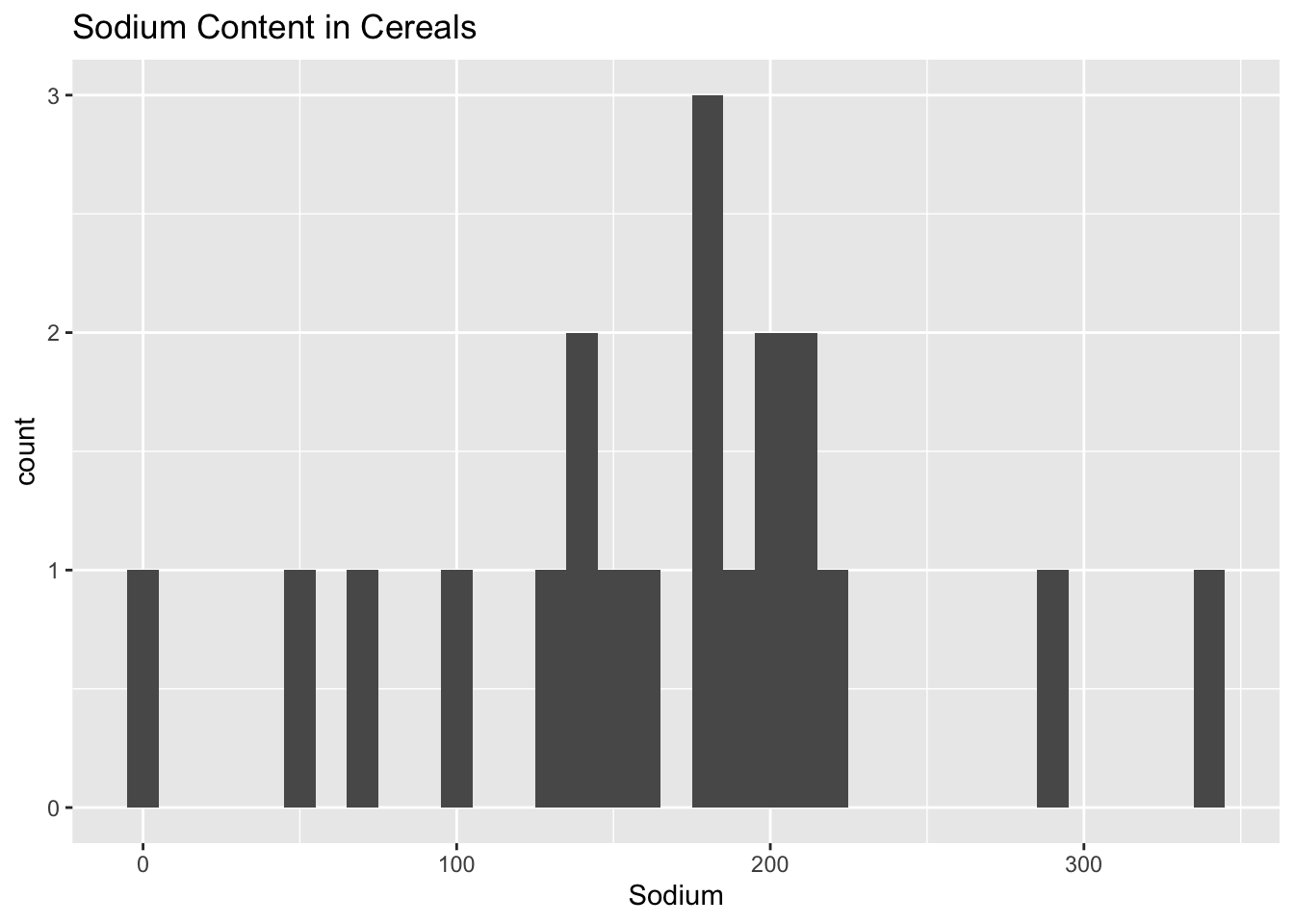
I chose to use a histogram here in order to get a general sense of the distribution of the data. It is helpful in order to see if there are any notable outliers that we should investigate further.
We can notice in this histogram that there are indeed a couple of outliers that have very low sodium and some that have very high sodium levels.
We can then compare this to the histogram of the sugar contents to see if there is a similar pattern.
ggplot(cereal, aes(x = Sugar)) + geom_histogram(binwidth = 9) + ggtitle("Sugar Content in Cereals")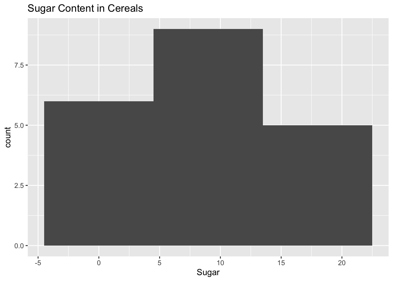
This histogram looks a lot more dense than the previous one. It doesn’t seem like there are any true outliers in terms of the sugar contents with most of the cereals having around a value of 10.
Bivariate Visualization(s)
One interesting visualization we could create is a scatter plot comparing the sugar contents of the cereals with the sodium contents. Additionally, in order for us to see if we can better understand what the variable Type means, we can color code the points based on their value for Type.
ggplot(data = cereal)+ geom_point(mapping = aes(x = Sodium, y = Sugar,col=Type)) + ggtitle("Sugar vs. Sodium Content in Cereals")
When we view the output of this plot, we can see that the majority of points fall in the middle of sodium with a couple of outliers to the side, while the cereals vary greatly on how much sugar they contain. This seems reasonable as most cereals aimed towards kids are very high in sugar, while cereals that are marketed towards adults are typically “healthy” and contain much less sugar.
Also we can note that it seems like Type C cereals are typically right in the middle of both sodium content and sugar content, while Type A cereals seem to be on the extremes of both categories.
I chose to use a scatter plot here as it is the best way for us to try and visually evaluate the correlation between two distinct variables. The scatter plot also lets us color the points based on a variable which lets us also try to get a better understanding of what the unknown variable Type represents.