Challenge 6

Visualizing Time and Relationships

library(tidyverse)
library(ggplot2)

knitr::opts_chunk$set(echo = TRUE, warning=FALSE, message=FALSE)

Introduction

I chose to use the fed_rate dataset for this challenge.

library(readr)
data <- read.csv("_data/FedFundsRate.csv")

ncol(data)

[1] 10

nrow(data)

[1] 904

Briefly describe the data

The dataset, FedFundsRate.csv, describes data collected from 1954 until 2017 of various macroeconomic indicators which are about the federal funds rate. The federal funds rate is the interest rate at which banks will lend money to each other to meet reserve requirements. The data contains 10 columns, 3 of which just display the date. 4 of the remaining variables are related to the federal funds rate (Federal Funds Upper Target,Effective Federal Funds Rate,Federal Funds Target Rate, and Federal Funds Lower Target). The final 3 variables are related to other economic statistics (Unemployment Rate, Inflation Rate, and Real GPD (Percent Channge)).

Tidy Data (as needed)

Many of the column names in the dataset are unnecessarily long so our first step in tidying this dataset is to rename all of those to something shorter and more readable.

library(dplyr)

data <- data %>%
  rename(Target_Rate = `Federal.Funds.Target.Rate`,
         Upper_Target = `Federal.Funds.Upper.Target`,
         Lower_Target = `Federal.Funds.Lower.Target`,
         Effective_Rate = `Effective.Federal.Funds.Rate`,
         GDP = `Real.GDP..Percent.Change.`,
         Unemployment_Rate = `Unemployment.Rate`,
         Inflation_Rate = `Inflation.Rate`)

# sanity check
colnames(data)

 [1] "Year"              "Month"             "Day"              
 [4] "Target_Rate"       "Upper_Target"      "Lower_Target"     
 [7] "Effective_Rate"    "GDP"               "Unemployment_Rate"
[10] "Inflation_Rate"   

We can also check to see if there are any missing values in the data

sum(is.na(data))

[1] 3196

As we can see, there are a lot of fields with missing values. However, there is at least one NA in every row so we cannot remove rows with missing values or else our dataset will be empty. For now, we will allow the NA’s to exist and will just ignore them when completing further investigations.

Another thing we could do is to mutate the date variables to be a single column.

data$date <- as.Date(paste(data$Year, data$Month, data$Day, sep = "-"))
data <- data %>%
  select(-Year, -Month, -Day)

Finally we can clean up this data by using the pivot_longer() command to make the date easier to use for our future investigations.

data <- data %>%
  pivot_longer(cols = -c(date), 
               names_to = "Variable", 
               values_to = "Value")

head(data) #sanity check

# A tibble: 6 × 3
  date       Variable          Value
  <date>     <chr>             <dbl>
1 1954-07-01 Target_Rate        NA  
2 1954-07-01 Upper_Target       NA  
3 1954-07-01 Lower_Target       NA  
4 1954-07-01 Effective_Rate      0.8
5 1954-07-01 GDP                 4.6
6 1954-07-01 Unemployment_Rate   5.8

Time Dependent Visualization

library(ggplot2)
fed_rate <- data %>% filter(Variable %in% c("Target_Rate", "Upper_Target", "Lower_Target", "Effective_Rate"))

ggplot(fed_rate, aes(x = date, y = Value, color = Variable)) + 
    geom_line() +
    labs(title = "Federal Funds Rate data over Time",
         x = "Date",
         y = "values") + theme_bw()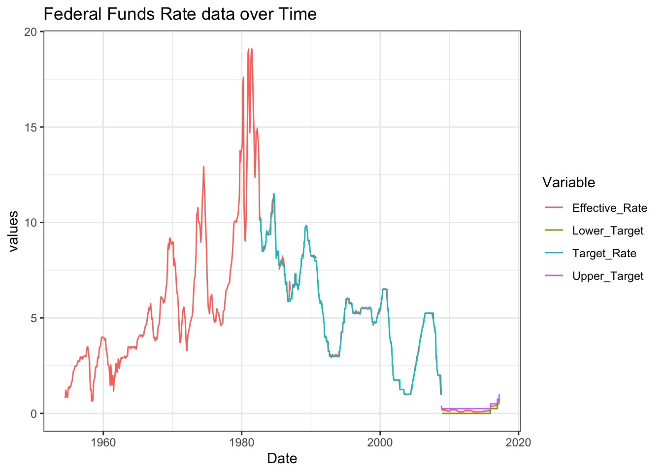

I chose to use this line graph as it shows us how closely the effective rate stays to the target over time.

Visualizing Part-Whole Relationships

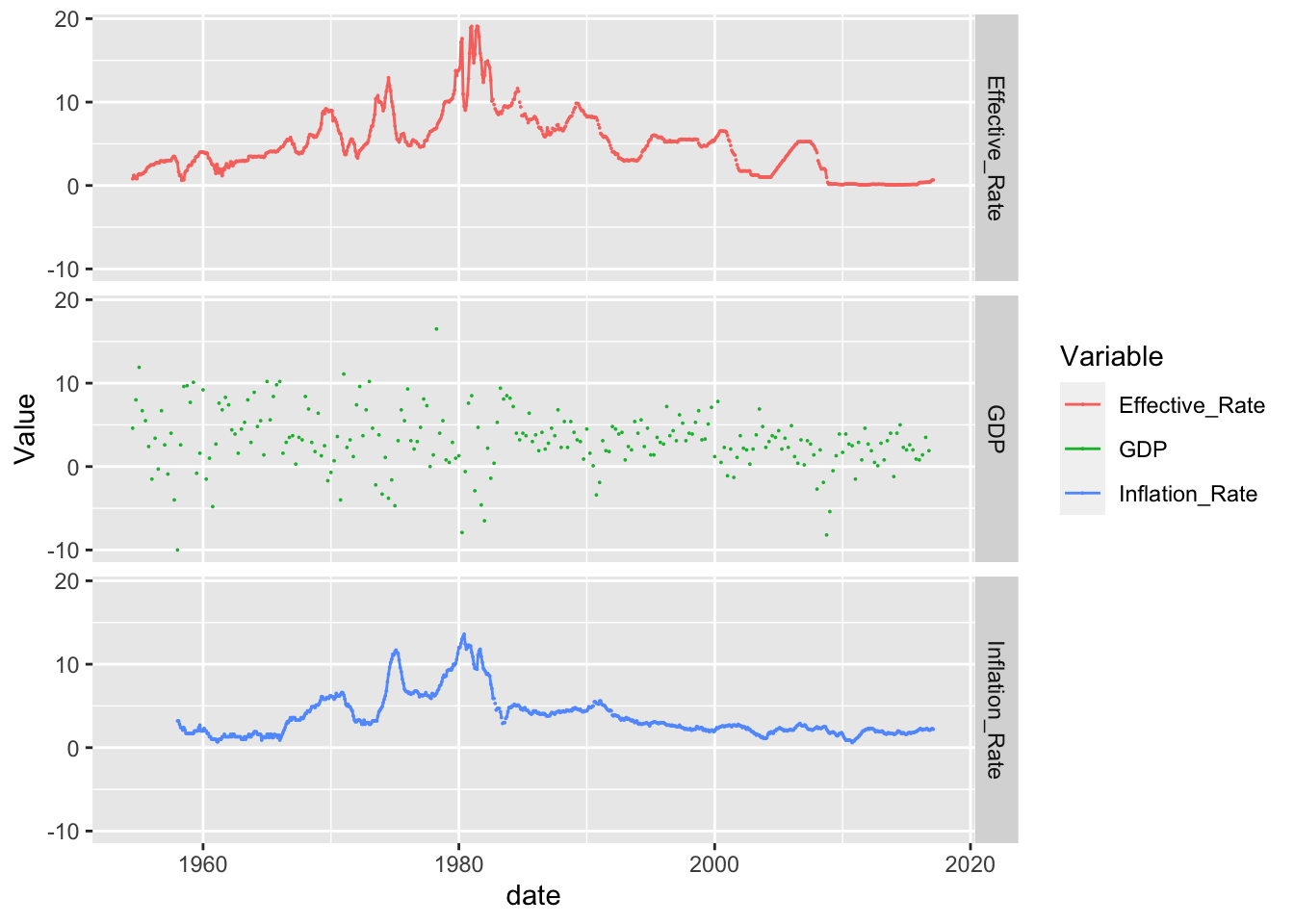
For this part, I chose to investigate how different variables changed alongside the effective federal funds rate. Using the facet_grid command allowed me to display these visualizations one after another which makes it easy to view how all variables are impacted over time.

data%>%
  filter(Variable%in%c("Effective_Rate", "GDP", 
                       "Unnemployment_Rate", "Inflation_Rate"))%>%
ggplot(., aes(x=date, y=Value, color=Variable))+
  geom_point(size=0)+
  geom_line()+
  facet_grid(rows = vars(Variable))