2019 AirBnB Rentals in NYC Boroughs

challenge_7

Michele Carlin

air_bnb

debt

Author

Michele Carlin

Published

April 19, 2023

Code

library(tidyverse)
library(summarytools)
library(dbplyr)
library(readxl)
library(readr)
library(ggplot2)
library(forcats)
library(scales)


knitr::opts_chunk$set(echo = TRUE)

Read in and view summary of ‘AB_NYC_2019’ dataset

Code

AB_NYC <- read_csv ("_data/AB_NYC_2019.csv")

Rows: 48895 Columns: 16
── Column specification ────────────────────────────────────────────────────────
Delimiter: ","
chr   (5): name, host_name, neighbourhood_group, neighbourhood, room_type
dbl  (10): id, host_id, latitude, longitude, price, minimum_nights, number_o...
date  (1): last_review

ℹ Use `spec()` to retrieve the full column specification for this data.
ℹ Specify the column types or set `show_col_types = FALSE` to quiet this message.

Code

View(AB_NYC)
view(dfSummary(AB_NYC))

Switching method to 'browser'
Output file written: C:\Users\CarlinML\AppData\Local\Temp\RtmpgxJwDt\file3ba467e3f04.html

This dataset contains 48895 rows and 16 columns. Each row/observation contains information on Airbnb rentals in NYC during 2019, including the type of rental (e.g., entire home, private room, shared room), the NYC borough, the price, minimum number of nights, and number of reviews.

Per the data frame summary, the price variable contains some $0’s; sort dataframe to review before recoding.

Code

arrange(AB_NYC, price)

# A tibble: 48,895 × 16
         id name   host_id host_…¹ neigh…² neigh…³ latit…⁴ longi…⁵ room_…⁶ price
      <dbl> <chr>    <dbl> <chr>   <chr>   <chr>     <dbl>   <dbl> <chr>   <dbl>
 1 18750597 Huge …  8.99e6 Kimber… Brookl… Bedfor…    40.7   -74.0 Privat…     0
 2 20333471 ★Host…  1.32e8 Anisha  Bronx   East M…    40.8   -73.9 Privat…     0
 3 20523843 MARTI…  1.58e7 Martia… Brookl… Bushwi…    40.7   -73.9 Privat…     0
 4 20608117 Sunny…  1.64e6 Lauren  Brookl… Greenp…    40.7   -73.9 Privat…     0
 5 20624541 Moder…  1.01e7 Aymeric Brookl… Willia…    40.7   -73.9 Entire…     0
 6 20639628 Spaci…  8.63e7 Adeyemi Brookl… Bedfor…    40.7   -73.9 Privat…     0
 7 20639792 Conte…  8.63e7 Adeyemi Brookl… Bedfor…    40.7   -73.9 Privat…     0
 8 20639914 Cozy …  8.63e7 Adeyemi Brookl… Bedfor…    40.7   -73.9 Privat…     0
 9 20933849 the b…  1.37e7 Qiuchi  Manhat… Murray…    40.8   -74.0 Entire…     0
10 21291569 Coliv…  1.02e8 Sergii  Brookl… Bushwi…    40.7   -73.9 Shared…     0
# … with 48,885 more rows, 6 more variables: minimum_nights <dbl>,
#   number_of_reviews <dbl>, last_review <date>, reviews_per_month <dbl>,
#   calculated_host_listings_count <dbl>, availability_365 <dbl>, and
#   abbreviated variable names ¹host_name, ²neighbourhood_group,
#   ³neighbourhood, ⁴latitude, ⁵longitude, ⁶room_type

Recode price=$0 to NA.

Code

AB_NYC <- AB_NYC %>% 
  mutate_at(c("price"), ~ na_if(., 0))

arrange(AB_NYC, price)

# A tibble: 48,895 × 16
         id name   host_id host_…¹ neigh…² neigh…³ latit…⁴ longi…⁵ room_…⁶ price
      <dbl> <chr>    <dbl> <chr>   <chr>   <chr>     <dbl>   <dbl> <chr>   <dbl>
 1  1620248 Large…  2.20e6 Sally   Manhat… East V…    40.7   -74.0 Entire…    10
 2 17437106 Couch…  3.35e7 Morgan  Manhat… Harlem     40.8   -74.0 Shared…    10
 3 17952277 Newly…  6.27e7 Katie   Brookl… Bushwi…    40.7   -73.9 Privat…    10
 4 17979764 Jen A…  8.45e7 Jennif… Manhat… SoHo       40.7   -74.0 Privat…    10
 5 18490141 IT'S …  9.70e7 Maria   Queens  Jamaica    40.7   -73.8 Entire…    10
 6 18835820 Quiet…  5.28e7 Amy     Manhat… Upper …    40.8   -74.0 Entire…    10
 7 19415314 Girls…  4.73e7 Mario   Manhat… Hell's…    40.8   -74.0 Shared…    10
 8 21869057 Spaci…  1.20e7 Vishan… Brookl… Greenp…    40.7   -74.0 Entire…    10
 9 24114389 Very …  1.81e8 Salim   Manhat… Upper …    40.8   -74.0 Privat…    10
10 24412104 Cozy …  9.10e7 Maureen Manhat… Kips B…    40.7   -74.0 Privat…    10
# … with 48,885 more rows, 6 more variables: minimum_nights <dbl>,
#   number_of_reviews <dbl>, last_review <date>, reviews_per_month <dbl>,
#   calculated_host_listings_count <dbl>, availability_365 <dbl>, and
#   abbreviated variable names ¹host_name, ²neighbourhood_group,
#   ³neighbourhood, ⁴latitude, ⁵longitude, ⁶room_type

Recode ‘price’ variable into new ‘price_range’ variable.

Code

AB_NYC <- AB_NYC %>%
  mutate(price_range = case_when(
         price < 100 ~ "less than $100",
         price >= 100 & price < 250 ~ "$100 - $249",
         price >= 250 & price < 500 ~ "$250 - $499",
         price >= 500 & price < 750 ~ "$500 - $749",
         price >= 750 & price < 1000 ~ "$750 - $999",
         price >= 1000 ~ "$1000 or more")
  )
AB_NYC %>% count(price_range)

# A tibble: 7 × 2
  price_range        n
  <chr>          <int>
1 $100 - $249    20792
2 $1000 or more    298
3 $250 - $499     4991
4 $500 - $749      682
5 $750 - $999      255
6 less than $100 21866
7 <NA>              11

Determine the values associated with each price range category.

Code

levels(factor(AB_NYC$price_range))

[1] "$100 - $249"    "$1000 or more"  "$250 - $499"    "$500 - $749"   
[5] "$750 - $999"    "less than $100"

Specify the factor order. I am having trouble re-ordering the factor levels on the graph.

Code

AB_NYC %>%
  filter (!is.na(price_range)) %>% 
 ggplot(aes(x=price_range)) + 
   geom_bar(position = "dodge",
           stat = "count", fill="purple", colour="black")+
   labs(title = "Frequency of Various Price Ranges", y = "Frequency", x = "Price Range")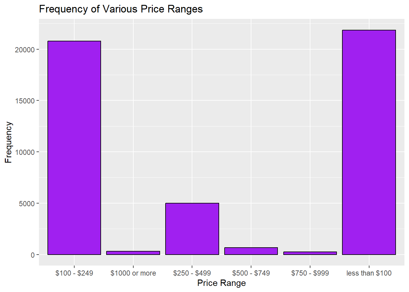

Code

AB_NYC %>%
 mutate(price_range_ordered = factor(price_range, levels = c(6,1,3,4,5,2))) %>%
 ggplot(aes(x=price_range_ordered)) + 
   geom_bar(position = "dodge", stat = "count", fill="purple", colour="black") +
   labs(title = "Frequency of Various Price Ranges", y = "Frequency", x = "Price Range")

Create ggplot of rentals by NYC Borough, order bars from highest to lowest value.

Code

AB_NYC %>%
 ggplot(aes(x=fct_infreq(neighbourhood_group))) + 
   geom_bar(stat = "count", fill="blue", colour="black")+
   labs(title = "AirBnB Rentals by NYC Borough", y = "Frequency", x = "NYC Borough")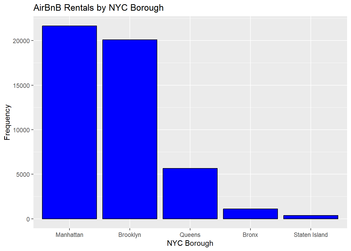

Calculate min/max/mean price (price) and group data by neighbourhood_group and room_type.

Code

GrpByNeighborhoodRoom <- AB_NYC %>%
    group_by(neighbourhood_group) %>%
    summarise(minADR = min(price, na.rm = TRUE), maxADR = max(price, na.rm = TRUE), meanADR = mean(price, na.rm = TRUE)) 
head(GrpByNeighborhoodRoom)

# A tibble: 5 × 4
  neighbourhood_group minADR maxADR meanADR
  <chr>                <dbl>  <dbl>   <dbl>
1 Bronx                   10   2500    87.6
2 Brooklyn                10  10000   124. 
3 Manhattan               10  10000   197. 
4 Queens                  10  10000    99.5
5 Staten Island           13   5000   115.

Code

AB_NYC %>%
 ggplot(aes(x=neighbourhood_group, y=price)) + 
   geom_bar(position = "dodge",fill="pink", colour="black",
           stat = "summary",
           fun = "mean")+
   labs(title = "Average AirBnB Nightly Cost by NYC Borough", y = "Average Nighyly Cost", x = "NYC Borough")

Warning: Removed 11 rows containing non-finite values (`stat_summary()`).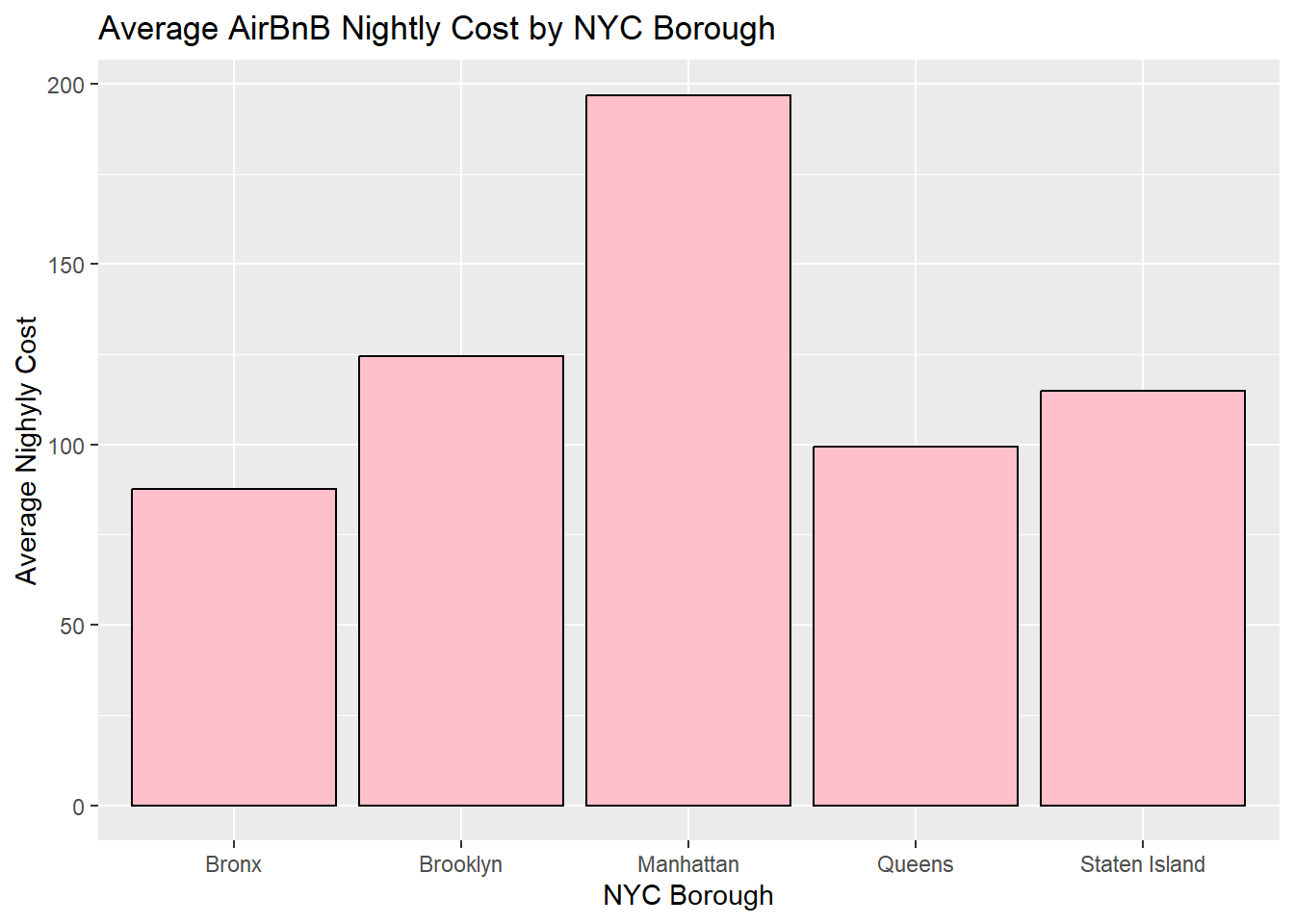

Adding facet wrap to graph.

Code

GrpByNeighborhoodRoom <- AB_NYC %>%
    group_by(neighbourhood_group, room_type) %>%
    summarise(minADR = min(price, na.rm = TRUE), maxADR = max(price, na.rm = TRUE), meanADR = mean(price, na.rm = TRUE))

`summarise()` has grouped output by 'neighbourhood_group'. You can override
using the `.groups` argument.

Code

head(GrpByNeighborhoodRoom)

# A tibble: 6 × 5
# Groups:   neighbourhood_group [2]
  neighbourhood_group room_type       minADR maxADR meanADR
  <chr>               <chr>            <dbl>  <dbl>   <dbl>
1 Bronx               Entire home/apt     28   1000   128. 
2 Bronx               Private room        10   2500    66.9
3 Bronx               Shared room         20    800    59.8
4 Brooklyn            Entire home/apt     10  10000   178. 
5 Brooklyn            Private room        10   7500    76.5
6 Brooklyn            Shared room         15    725    50.8

Code

tail(GrpByNeighborhoodRoom)

# A tibble: 6 × 5
# Groups:   neighbourhood_group [2]
  neighbourhood_group room_type       minADR maxADR meanADR
  <chr>               <chr>            <dbl>  <dbl>   <dbl>
1 Queens              Entire home/apt     10   2600   147. 
2 Queens              Private room        10  10000    71.8
3 Queens              Shared room         11   1800    69.0
4 Staten Island       Entire home/apt     48   5000   174. 
5 Staten Island       Private room        20    300    62.3
6 Staten Island       Shared room         13    150    57.4

Code

AB_NYC %>%
ggplot(aes(x=neighbourhood_group, y=price, fill=room_type)) + 
   geom_bar(position = "dodge",
           stat = "summary",
           fun = "mean")+
   facet_wrap(vars(room_type), scales = "free_x") +
  scale_fill_manual(values=c("green","orange","blue"))+
  theme(legend.position="none")+
   scale_x_discrete(guide = guide_axis(n.dodge=2))+
   labs(title = "Average AirBnB Nightly Cost by NYC Borough and Room Type", y = "Average Nightly Cost", x = "NYC Borough")

Warning: Removed 11 rows containing non-finite values (`stat_summary()`).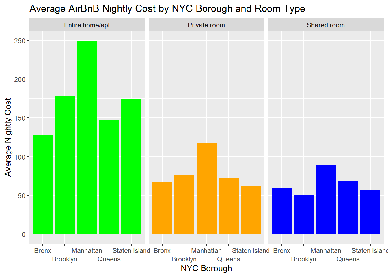

Code

AB_NYC %>%
  ggplot(aes(fill=price_range, x=room_type)) + 
    geom_bar(position="dodge", stat="count")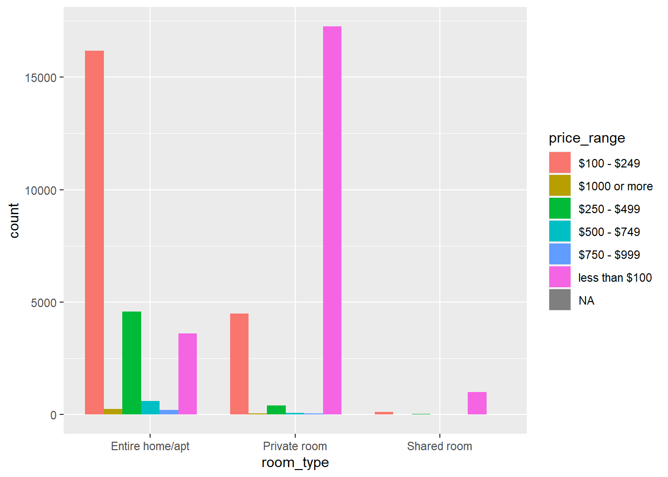

Read in and view summary of ‘debt_in_trillions’ dataset.

Code

sheet_names <- excel_sheets("_data/debt_in_trillions.xlsx")
sheet_names

[1] "Sheet1"

Code

debt_trillions <- read_xlsx ("_data/debt_in_trillions.xlsx")
View(debt_trillions)
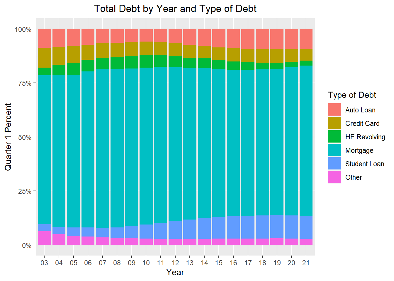
view(dfSummary(debt_trillions))

Switching method to 'browser'

Output file written: C:\Users\CarlinML\AppData\Local\Temp\RtmpgxJwDt\file3ba456825d96.html

This dataset contains 74 rows and 8 columns. Each row represents a particular year/quarter and provides the average debt in trillions for various types of household expenses (e.g., mortgage, auto loan, credit card, etc.).

Pivot longer so that each row contains one observation.

Code

debt_trillions_long <- pivot_longer(debt_trillions, col = c(Mortgage, 'HE Revolving', 'Auto Loan', 'Credit Card', 'Student Loan', Other, Total),
                 names_to="debt_type",
                 values_to = "value")
View(debt_trillions_long)
view(dfSummary(debt_trillions_long))

Switching method to 'browser'

Output file written: C:\Users\CarlinML\AppData\Local\Temp\RtmpgxJwDt\file3ba418dc7fec.html

Separate ‘Year and Quarter’ into two variables.

Code

debt_trillions_long <- debt_trillions_long %>%
  separate("Year and Quarter", c("year", "quarter"), ":")
view(dfSummary(debt_trillions_long))

Switching method to 'browser'

Output file written: C:\Users\CarlinML\AppData\Local\Temp\RtmpgxJwDt\file3ba43eca7d1b.html

Create stacked bar chart of debt type by year for quarter 1 only.

Code

theme_update(plot.title = element_text(hjust = 0.5))

debt_trillions_long %>%
  mutate(debt_type = factor(debt_type, levels=c("Auto Loan", "Credit Card", "HE Revolving", "Mortgage", "Student Loan", "Other"))) %>%
  filter(debt_type != 'Total') %>%
  ggplot(aes(x = year, y = value, fill = debt_type)) +
  geom_col(position = "fill") +
  scale_y_continuous(labels = percent) +
  labs(title = "Total Debt by Year and Type of Debt", y = "Quarter 1 Percent", x = "Year", fill="Type of Debt")