library(tidyverse)
library(ggplot2)

knitr::opts_chunk$set(echo = TRUE, warning=FALSE, message=FALSE)
Challenge 7
challenge_7
hotel_bookings
poobigan murugesan
Visualizing Multiple Dimensions
Challenge Overview
Today’s challenge is to:
- read in a data set, and describe the data set using both words and any supporting information (e.g., tables, etc)
- tidy data (as needed, including sanity checks)
- mutate variables as needed (including sanity checks)
- Recreate at least two graphs from previous exercises, but introduce at least one additional dimension that you omitted before using ggplot functionality (color, shape, line, facet, etc) The goal is not to create unneeded chart ink (Tufte), but to concisely capture variation in additional dimensions that were collapsed in your earlier 2 or 3 dimensional graphs.
- Explain why you choose the specific graph type
- If you haven’t tried in previous weeks, work this week to make your graphs “publication” ready with titles, captions, and pretty axis labels and other viewer-friendly features
R Graph Gallery is a good starting point for thinking about what information is conveyed in standard graph types, and includes example R code. And anyone not familiar with Edward Tufte should check out his fantastic books and courses on data visualizaton.
(be sure to only include the category tags for the data you use!)
Read in data
df<-read.csv("_data/hotel_bookings.csv")Summary
dim(df)[1] 119390 32summary(df) hotel is_canceled lead_time arrival_date_year
Length:119390 Min. :0.0000 Min. : 0 Min. :2015
Class :character 1st Qu.:0.0000 1st Qu.: 18 1st Qu.:2016
Mode :character Median :0.0000 Median : 69 Median :2016
Mean :0.3704 Mean :104 Mean :2016
3rd Qu.:1.0000 3rd Qu.:160 3rd Qu.:2017
Max. :1.0000 Max. :737 Max. :2017
arrival_date_month arrival_date_week_number arrival_date_day_of_month
Length:119390 Min. : 1.00 Min. : 1.0
Class :character 1st Qu.:16.00 1st Qu.: 8.0
Mode :character Median :28.00 Median :16.0
Mean :27.17 Mean :15.8
3rd Qu.:38.00 3rd Qu.:23.0
Max. :53.00 Max. :31.0
stays_in_weekend_nights stays_in_week_nights adults
Min. : 0.0000 Min. : 0.0 Min. : 0.000
1st Qu.: 0.0000 1st Qu.: 1.0 1st Qu.: 2.000
Median : 1.0000 Median : 2.0 Median : 2.000
Mean : 0.9276 Mean : 2.5 Mean : 1.856
3rd Qu.: 2.0000 3rd Qu.: 3.0 3rd Qu.: 2.000
Max. :19.0000 Max. :50.0 Max. :55.000
children babies meal country
Min. : 0.0000 Min. : 0.000000 Length:119390 Length:119390
1st Qu.: 0.0000 1st Qu.: 0.000000 Class :character Class :character
Median : 0.0000 Median : 0.000000 Mode :character Mode :character
Mean : 0.1039 Mean : 0.007949
3rd Qu.: 0.0000 3rd Qu.: 0.000000
Max. :10.0000 Max. :10.000000
NA's :4
market_segment distribution_channel is_repeated_guest
Length:119390 Length:119390 Min. :0.00000
Class :character Class :character 1st Qu.:0.00000
Mode :character Mode :character Median :0.00000
Mean :0.03191
3rd Qu.:0.00000
Max. :1.00000
previous_cancellations previous_bookings_not_canceled reserved_room_type
Min. : 0.00000 Min. : 0.0000 Length:119390
1st Qu.: 0.00000 1st Qu.: 0.0000 Class :character
Median : 0.00000 Median : 0.0000 Mode :character
Mean : 0.08712 Mean : 0.1371
3rd Qu.: 0.00000 3rd Qu.: 0.0000
Max. :26.00000 Max. :72.0000
assigned_room_type booking_changes deposit_type agent
Length:119390 Min. : 0.0000 Length:119390 Length:119390
Class :character 1st Qu.: 0.0000 Class :character Class :character
Mode :character Median : 0.0000 Mode :character Mode :character
Mean : 0.2211
3rd Qu.: 0.0000
Max. :21.0000
company days_in_waiting_list customer_type adr
Length:119390 Min. : 0.000 Length:119390 Min. : -6.38
Class :character 1st Qu.: 0.000 Class :character 1st Qu.: 69.29
Mode :character Median : 0.000 Mode :character Median : 94.58
Mean : 2.321 Mean : 101.83
3rd Qu.: 0.000 3rd Qu.: 126.00
Max. :391.000 Max. :5400.00
required_car_parking_spaces total_of_special_requests reservation_status
Min. :0.00000 Min. :0.0000 Length:119390
1st Qu.:0.00000 1st Qu.:0.0000 Class :character
Median :0.00000 Median :0.0000 Mode :character
Mean :0.06252 Mean :0.5714
3rd Qu.:0.00000 3rd Qu.:1.0000
Max. :8.00000 Max. :5.0000
reservation_status_date
Length:119390
Class :character
Mode :character
Briefly describe the data
The dataset contains data on hotel bookings and comprises a total of 119,390 entries. It encompasses various information, including hotel type, cancellation status, lead time, arrival date (year, month, day), duration of stay, number of adults, children, and babies, meal preferences, country of origin, market segment, distribution channel, previous cancellations, reserved and assigned room types, booking changes, deposit type, days on the waiting list, customer type, average daily rate, required car parking spaces, and total number of special requests.
Unique countries in dataset (178)
df$country%>%unique() [1] "PRT" "GBR" "USA" "ESP" "IRL" "FRA" "NULL" "ROU" "NOR" "OMN"
[11] "ARG" "POL" "DEU" "BEL" "CHE" "CN" "GRC" "ITA" "NLD" "DNK"
[21] "RUS" "SWE" "AUS" "EST" "CZE" "BRA" "FIN" "MOZ" "BWA" "LUX"
[31] "SVN" "ALB" "IND" "CHN" "MEX" "MAR" "UKR" "SMR" "LVA" "PRI"
[41] "SRB" "CHL" "AUT" "BLR" "LTU" "TUR" "ZAF" "AGO" "ISR" "CYM"
[51] "ZMB" "CPV" "ZWE" "DZA" "KOR" "CRI" "HUN" "ARE" "TUN" "JAM"
[61] "HRV" "HKG" "IRN" "GEO" "AND" "GIB" "URY" "JEY" "CAF" "CYP"
[71] "COL" "GGY" "KWT" "NGA" "MDV" "VEN" "SVK" "FJI" "KAZ" "PAK"
[81] "IDN" "LBN" "PHL" "SEN" "SYC" "AZE" "BHR" "NZL" "THA" "DOM"
[91] "MKD" "MYS" "ARM" "JPN" "LKA" "CUB" "CMR" "BIH" "MUS" "COM"
[101] "SUR" "UGA" "BGR" "CIV" "JOR" "SYR" "SGP" "BDI" "SAU" "VNM"
[111] "PLW" "QAT" "EGY" "PER" "MLT" "MWI" "ECU" "MDG" "ISL" "UZB"
[121] "NPL" "BHS" "MAC" "TGO" "TWN" "DJI" "STP" "KNA" "ETH" "IRQ"
[131] "HND" "RWA" "KHM" "MCO" "BGD" "IMN" "TJK" "NIC" "BEN" "VGB"
[141] "TZA" "GAB" "GHA" "TMP" "GLP" "KEN" "LIE" "GNB" "MNE" "UMI"
[151] "MYT" "FRO" "MMR" "PAN" "BFA" "LBY" "MLI" "NAM" "BOL" "PRY"
[161] "BRB" "ABW" "AIA" "SLV" "DMA" "PYF" "GUY" "LCA" "ATA" "GTM"
[171] "ASM" "MRT" "NCL" "KIR" "SDN" "ATF" "SLE" "LAO" Unique hotels in dataset (2)
df$hotel%>%unique()[1] "Resort Hotel" "City Hotel" df$arrival_date_year %>%unique()[1] 2015 2016 2017Tidy Data (as needed)
To observe the reservations trend over time, we merge all the relevant fields(date, month, year) into a single date field. However, we will keep the “arrival_month” field unchanged in order to visualize the monthly trend.
df$date <- as.Date(paste(df$arrival_date_year, df$arrival_date_month, df$arrival_date_day_of_month, sep = "-"), format = "%Y-%B-%d")
df$date %>% head()
[1] "2015-07-01" "2015-07-01" "2015-07-01" "2015-07-01" "2015-07-01"
[6] "2015-07-01"Visualization with Multiple Dimensions
In challenge 6 we visualized the trend of number of reservations for a hotel, here we add fill type for hotels thus adding a dimension. We use a histogram since it excels at providing a visual summary of count data, aiding in the exploration, comparison, and interpretation of distributions, making it an outstanding choice for data analysis and visualization. Number of reservations trend:
df_plot2 <-df %>%
                  group_by(date, hotel)%>%
                  summarise(count = n())

ggplot(df_plot2) +labs(title = "Number of reservations trend")+
  geom_bar(aes(x=date, y=count, fill=hotel), stat = "identity")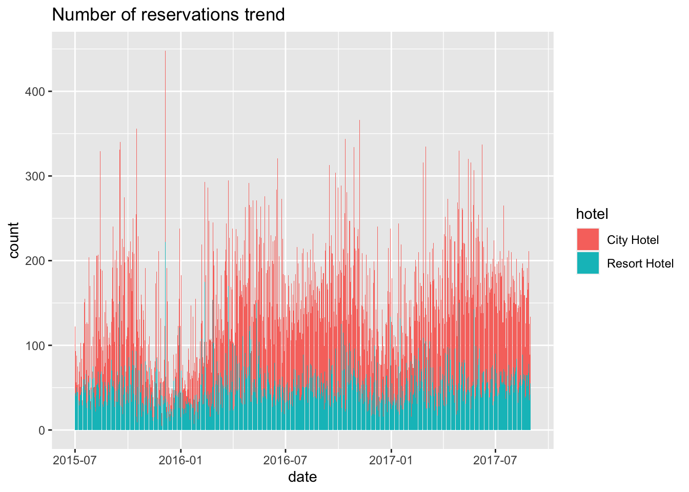
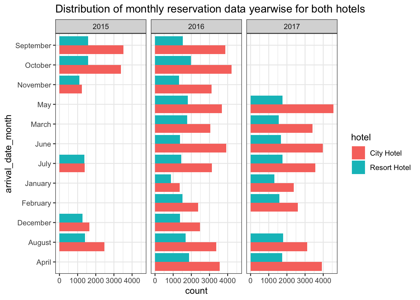
Recreating the second graph from previous assignment but using a bar plot instead of a line to show better distinction and adding a year dimension
df_plot <-df %>%
                                  group_by(arrival_date_month, hotel, arrival_date_year) %>%
                                  summarise(count = n())

ggplot(df_plot) + geom_bar(aes(x = arrival_date_month, y = count, fill = hotel ), stat="identity", position = "dodge")+theme_bw() + facet_grid(~arrival_date_year)+ coord_flip()+labs(title = "Distribution of monthly reservation data yearwise for both hotels")