Challenge 8

challenge_8

snl

Joining Data

Author

Pooja Shah

Published

April 29, 2023

library(tidyverse)
library(ggplot2)
library(dplyr)

knitr::opts_chunk$set(echo = TRUE, warning=FALSE, message=FALSE)

Challenge Overview

Today’s challenge is to:

read in multiple data sets, and describe the data set using both words and any supporting information (e.g., tables, etc)
tidy data (as needed, including sanity checks)
mutate variables as needed (including sanity checks)
join two or more data sets and analyze some aspect of the joined data

(be sure to only include the category tags for the data you use!)

Read in data

Read in one (or more) of the following datasets, using the correct R package and command.

military marriages ⭐⭐
faostat ⭐⭐
railroads ⭐⭐⭐
fed_rate ⭐⭐⭐
debt ⭐⭐⭐
us_hh ⭐⭐⭐⭐
snl ⭐⭐⭐⭐⭐

snl_actors <- read_csv("_data/snl_actors.csv")
head(snl_actors)

# A tibble: 6 × 4
  aid            url           type  gender 
  <chr>          <chr>         <chr> <chr>  
1 Kate McKinnon  /Cast/?KaMc   cast  female 
2 Alex Moffat    /Cast/?AlMo   cast  male   
3 Ego Nwodim     /Cast/?EgNw   cast  unknown
4 Chris Redd     /Cast/?ChRe   cast  male   
5 Kenan Thompson /Cast/?KeTh   cast  male   
6 Carey Mulligan /Guests/?3677 guest andy

snl_casts <- read_csv("_data/snl_casts.csv")
head(snl_casts)

# A tibble: 6 × 8
  aid                sid featured first_epid last_epid update_anchor n_episodes
  <chr>            <dbl> <lgl>         <dbl>     <dbl> <lgl>              <dbl>
1 A. Whitney Brown    11 TRUE       19860222        NA FALSE                  8
2 A. Whitney Brown    12 TRUE             NA        NA FALSE                 20
3 A. Whitney Brown    13 TRUE             NA        NA FALSE                 13
4 A. Whitney Brown    14 TRUE             NA        NA FALSE                 20
5 A. Whitney Brown    15 TRUE             NA        NA FALSE                 20
6 A. Whitney Brown    16 TRUE             NA        NA FALSE                 20
# ℹ 1 more variable: season_fraction <dbl>

snl_seasons <- read_csv("_data/snl_seasons.csv")
head(snl_seasons)

# A tibble: 6 × 5
    sid  year first_epid last_epid n_episodes
  <dbl> <dbl>      <dbl>     <dbl>      <dbl>
1     1  1975   19751011  19760731         24
2     2  1976   19760918  19770521         22
3     3  1977   19770924  19780520         20
4     4  1978   19781007  19790526         20
5     5  1979   19791013  19800524         20
6     6  1980   19801115  19810411         13

Briefly describe the data

Tidy Data (as needed)

Is your data already tidy, or is there work to be done? Be sure to anticipate your end result to provide a sanity check, and document your work here.

snl_actors <- snl_actors %>%
  drop_na()
snl_actors

# A tibble: 2,249 × 4
   aid            url           type  gender 
   <chr>          <chr>         <chr> <chr>  
 1 Kate McKinnon  /Cast/?KaMc   cast  female 
 2 Alex Moffat    /Cast/?AlMo   cast  male   
 3 Ego Nwodim     /Cast/?EgNw   cast  unknown
 4 Chris Redd     /Cast/?ChRe   cast  male   
 5 Kenan Thompson /Cast/?KeTh   cast  male   
 6 Carey Mulligan /Guests/?3677 guest andy   
 7 Marcus Mumford /Guests/?3679 guest male   
 8 Aidy Bryant    /Cast/?AiBr   cast  female 
 9 Steve Higgins  /Crew/?StHi   crew  male   
10 Mikey Day      /Cast/?MiDa   cast  male   
# ℹ 2,239 more rows

snl_casts <- snl_casts %>%
  select(aid, sid, featured, update_anchor, n_episodes, season_fraction)
snl_casts <- snl_casts %>%
  drop_na()
snl_casts

# A tibble: 614 × 6
   aid                sid featured update_anchor n_episodes season_fraction
   <chr>            <dbl> <lgl>    <lgl>              <dbl>           <dbl>
 1 A. Whitney Brown    11 TRUE     FALSE                  8           0.444
 2 A. Whitney Brown    12 TRUE     FALSE                 20           1    
 3 A. Whitney Brown    13 TRUE     FALSE                 13           1    
 4 A. Whitney Brown    14 TRUE     FALSE                 20           1    
 5 A. Whitney Brown    15 TRUE     FALSE                 20           1    
 6 A. Whitney Brown    16 TRUE     FALSE                 20           1    
 7 Alan Zweibel         5 TRUE     FALSE                  5           0.25 
 8 Sasheer Zamata      39 TRUE     FALSE                 11           0.524
 9 Sasheer Zamata      40 TRUE     FALSE                 21           1    
10 Sasheer Zamata      41 FALSE    FALSE                 21           1    
# ℹ 604 more rows

snl_seasons <- snl_seasons %>% 
  drop_na()
snl_seasons

# A tibble: 46 × 5
     sid  year first_epid last_epid n_episodes
   <dbl> <dbl>      <dbl>     <dbl>      <dbl>
 1     1  1975   19751011  19760731         24
 2     2  1976   19760918  19770521         22
 3     3  1977   19770924  19780520         20
 4     4  1978   19781007  19790526         20
 5     5  1979   19791013  19800524         20
 6     6  1980   19801115  19810411         13
 7     7  1981   19811003  19820522         20
 8     8  1982   19820925  19830514         20
 9     9  1983   19831008  19840512         19
10    10  1984   19841006  19850413         17
# ℹ 36 more rows

Are there any variables that require mutation to be usable in your analysis stream? For example, do you need to calculate new values in order to graph them? Can string values be represented numerically? Do you need to turn any variables into factors and reorder for ease of graphics and visualization?

Document your work here.

colnames(snl_actors)

[1] "aid"    "url"    "type"   "gender"

colnames(snl_casts)

[1] "aid"             "sid"             "featured"        "update_anchor"  
[5] "n_episodes"      "season_fraction"

colnames(snl_seasons)

[1] "sid"        "year"       "first_epid" "last_epid"  "n_episodes"

snl_season <- snl_seasons %>%
  select(sid, year)

snl_cast <- snl_casts %>%
  select(aid, sid, n_episodes)

Join Data

Be sure to include a sanity check, and double-check that case count is correct!

snl_data <- snl_casts %>%
  select(-update_anchor, -season_fraction, -n_episodes) %>%
  left_join(snl_season, by="sid")

snl_data

# A tibble: 614 × 4
   aid                sid featured  year
   <chr>            <dbl> <lgl>    <dbl>
 1 A. Whitney Brown    11 TRUE      1985
 2 A. Whitney Brown    12 TRUE      1986
 3 A. Whitney Brown    13 TRUE      1987
 4 A. Whitney Brown    14 TRUE      1988
 5 A. Whitney Brown    15 TRUE      1989
 6 A. Whitney Brown    16 TRUE      1990
 7 Alan Zweibel         5 TRUE      1979
 8 Sasheer Zamata      39 TRUE      2013
 9 Sasheer Zamata      40 TRUE      2014
10 Sasheer Zamata      41 FALSE     2015
# ℹ 604 more rows

#Graph representing aid and which years they worked in

ggplot(snl_data, aes(aid)) +
  geom_bar() +
  labs(title = "Graph showing how many season each aid worked for")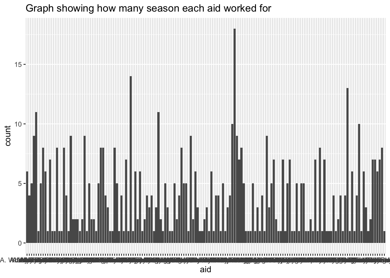

snl_data1 <- snl_actors %>%
  select(-url) %>%
  inner_join(snl_cast, by="aid")

snl_data1

# A tibble: 607 × 5
   aid           type  gender   sid n_episodes
   <chr>         <chr> <chr>  <dbl>      <dbl>
 1 Kate McKinnon cast  female    37          5
 2 Kate McKinnon cast  female    38         21
 3 Kate McKinnon cast  female    39         21
 4 Kate McKinnon cast  female    40         21
 5 Kate McKinnon cast  female    41         21
 6 Kate McKinnon cast  female    42         21
 7 Kate McKinnon cast  female    43         21
 8 Kate McKinnon cast  female    44         21
 9 Kate McKinnon cast  female    45         18
10 Kate McKinnon cast  female    46         17
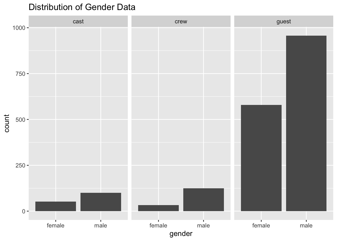
# ℹ 597 more rows

gender_data <- snl_actors %>%
  filter(gender == "male" | gender == "female")

snl_data1 %>%
  filter(type == "cast") %>%
  ggplot(aes(sid, fill=gender)) +
  geom_bar() +
  labs(title = "Distribution of Cast per Season by Gender")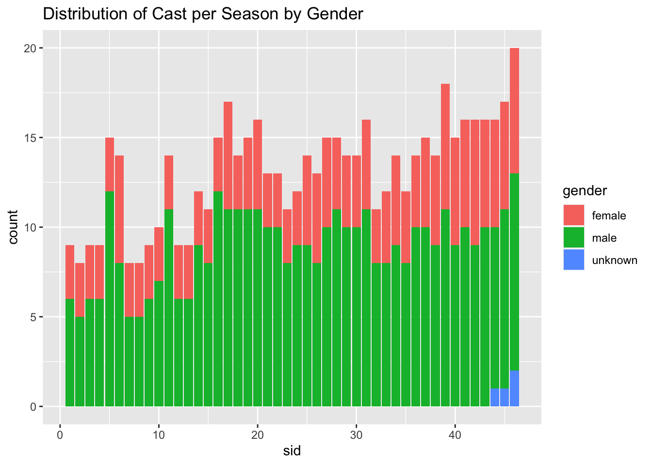

ggplot(gender_data, aes(gender)) +
  geom_bar() +
  facet_wrap(vars(type)) +
  labs(title = "Distribution of Gender Data")