library(tidyverse)
library(ggplot2)
library(tidyr)
library(dplyr)
knitr::opts_chunk$set(echo = TRUE, warning=FALSE, message=FALSE)Final Project Assignment#1: Project & Data Description
final_Project_assignment_1
final_project_data_description
Project & Data Description
Introduction
Dataset(s) Introduction:
I will be using a kaggle dataset about Superstore Sales for Sales Forecasting. The dataset has information about sales in a retail store and I will use that data to forecast sales pattern.
The dataset has almost 10k rows of information about sales and their 18 attributes. Each row consists of information such as the ordered goods information, shipment information, customer information and sales information.
What questions do you like to answer with this dataset(s)?
My main aim with this dataset is to understand the trends within the data and predict on the amount of goods that will be sold in the nearby future.
This will lead to knowing how much surplus amount of goods a company should have ready to make sure there isn’t a shortage in the stores in the future.
Describe the data set(s)
- displaying the data
data <- read_csv("PoojaShah_FinalProjectData/_data/data.csv")
data- descriptive information of the dataset
dim(data)[1] 9800 18colnames(data) [1] "Row ID" "Order ID" "Order Date" "Ship Date"
[5] "Ship Mode" "Customer ID" "Customer Name" "Segment"
[9] "Country" "City" "State" "Postal Code"
[13] "Region" "Product ID" "Category" "Sub-Category"
[17] "Product Name" "Sales" # Modifying Column Names
colnames(data)[3] = "OrderDate"
colnames(data)[5] = "ShipMode"
colnames(data)[16] = "SubCategory"
colnames(data) [1] "Row ID" "Order ID" "OrderDate" "Ship Date"
[5] "ShipMode" "Customer ID" "Customer Name" "Segment"
[9] "Country" "City" "State" "Postal Code"
[13] "Region" "Product ID" "Category" "SubCategory"
[17] "Product Name" "Sales" - cleaning the data;
# Modifying data to split dates
dateData <- data %>%
separate_wider_delim(OrderDate, '/', names = c("Date", "Month", "Year"))
dateDatadateData$Month = as.numeric(as.character(dateData$Month))
dateData$Year = as.numeric(as.character(dateData$Year))
# Making a new dataframe with only necessary colums
newData <- dateData %>%
select(c("Month", "Year", "ShipMode", "Segment", "Country", "State", "Region", "Category", "SubCategory", "Sales"))
newData- summary statistics of data:
summary(newData) Month Year ShipMode Segment
Min. : 1.000 Min. :2015 Length:9800 Length:9800
1st Qu.: 5.000 1st Qu.:2016 Class :character Class :character
Median : 9.000 Median :2017 Mode :character Mode :character
Mean : 7.818 Mean :2017
3rd Qu.:11.000 3rd Qu.:2018
Max. :12.000 Max. :2018
Country State Region Category
Length:9800 Length:9800 Length:9800 Length:9800
Class :character Class :character Class :character Class :character
Mode :character Mode :character Mode :character Mode :character
SubCategory Sales
Length:9800 Min. : 0.444
Class :character 1st Qu.: 17.248
Mode :character Median : 54.490
Mean : 230.769
3rd Qu.: 210.605
Max. :22638.480 newData %>%
select(Sales) %>%
sapply(sd) Sales
626.6519 Storytelling Component
#you should describe the basic information of the dataset(s) and the variables in a way that corresponds to your descriptive and summary statistics in the above coding component
- Here, I am using 10 columns of the data that seemed important for my analysis. These columns are as under:
colnames(newData) [1] "Month" "Year" "ShipMode" "Segment" "Country"
[6] "State" "Region" "Category" "SubCategory" "Sales" - For example, suppose I use a dataset of all the athletes who participated in the Olympic Games. Here is how I describe the basic information of the data: “the case of this dataset is ab individual athlete, represented by each row in the dataset. The dataset includes individual (e.g., gender, age, height, weight, race) and event performance (e.g., final placement) information for all athletes (22,398) competing in all events (e.g., Male 400m Free, Female …) in all Olympics Games since 1922 (24 Winter and 28 Summer Games. Athletes appearing in the dataset competed in anywhere from 1-11 distinct events (of 198 possible) during 1-5 distinct Olympic competitions, for a total of XXX, XXX athlete-event-Olympic-year observations. XXX Countries are represented, etc).”
3. Visualization
- Briefly describe what data analyses (please the special note on statistics in the next section) and visualizations you plan to conduct to answer the research questions you proposed above.
ggplot(data, aes(Region, fill = Segment)) +
geom_bar() +
labs(title = "Sales per Region by Segment") 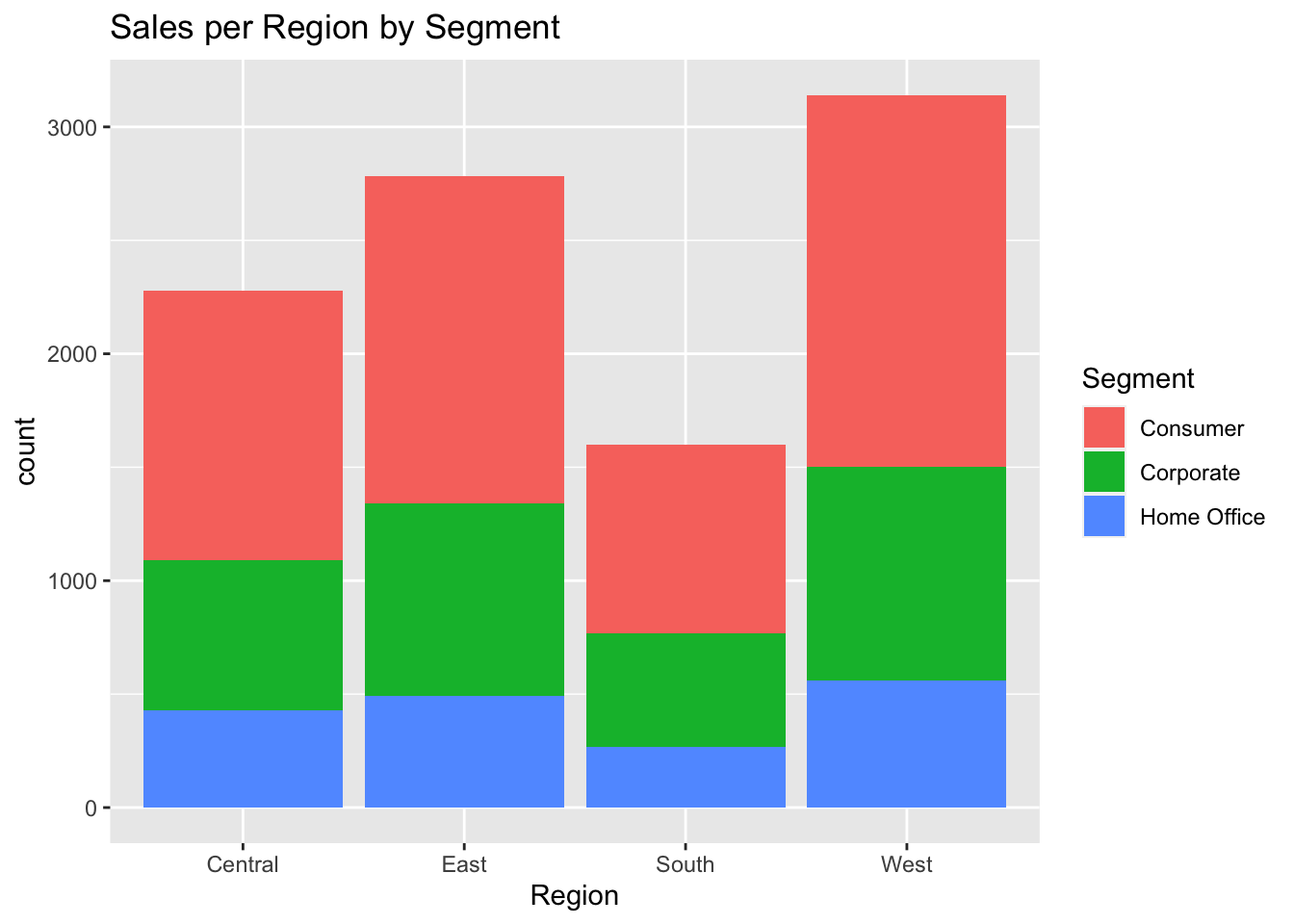
ggplot(data, aes(Region, fill = Segment)) +
geom_bar() +
labs(title = "Sales per Region by Segment divided by States") +
facet_wrap(vars(State)) 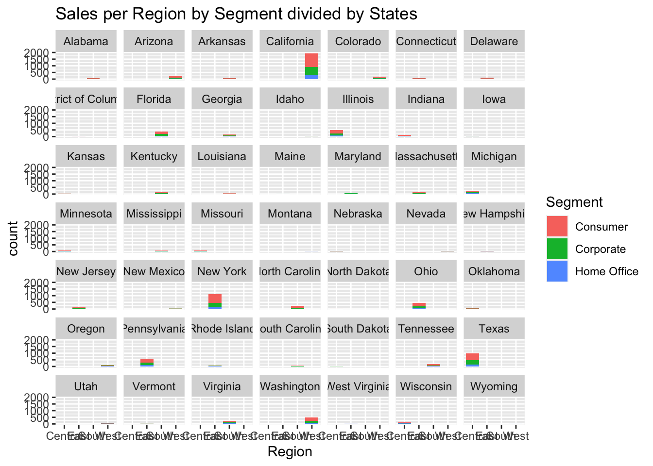
ggplot(data, aes(Category, fill = Segment)) +
geom_bar() +
labs(title = "Sales by Category per Segment")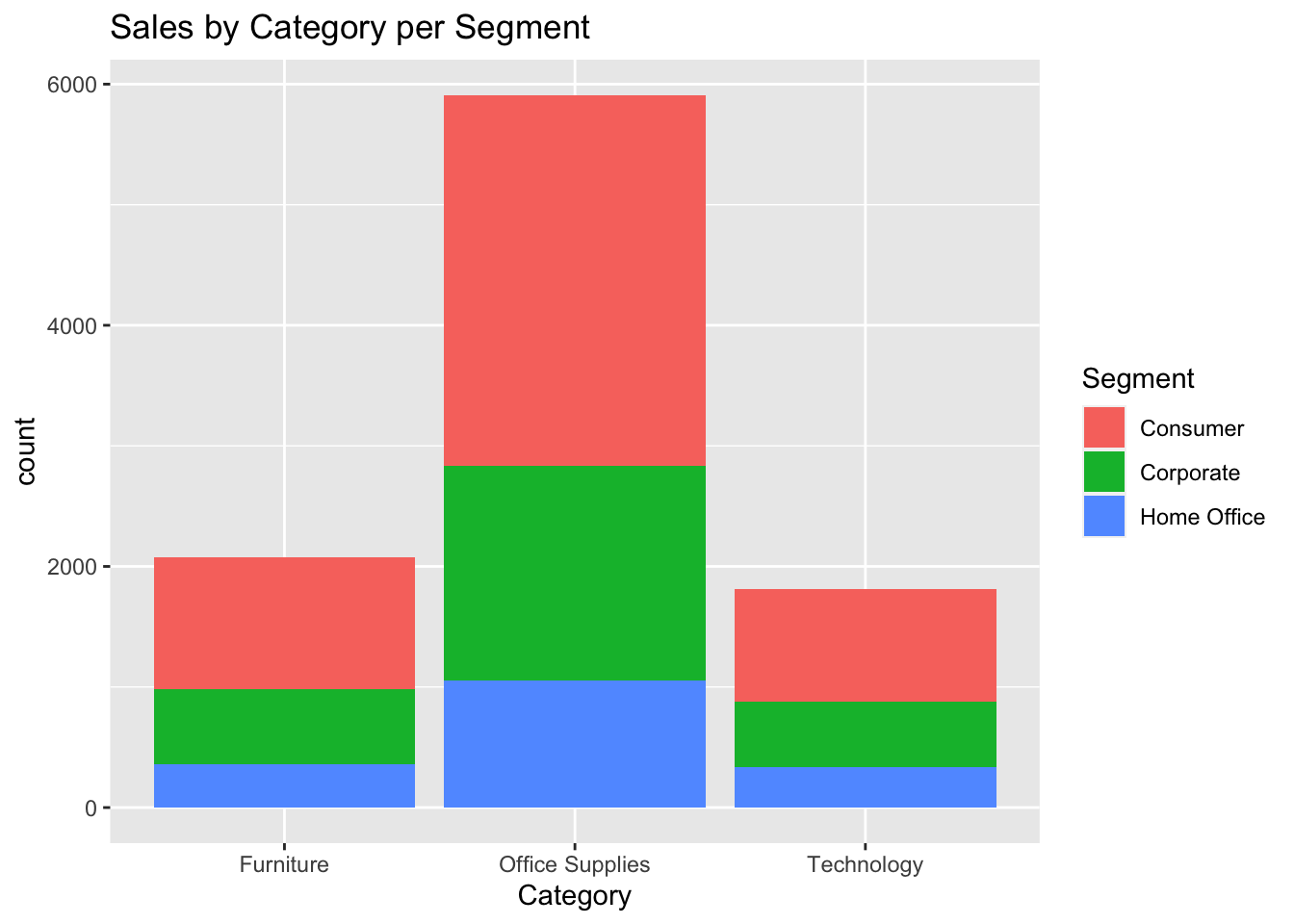
ggplot(data, aes(Category)) +
geom_bar() +
labs(title = "Sales by SubCategory per Segment") +
facet_wrap(vars(Segment))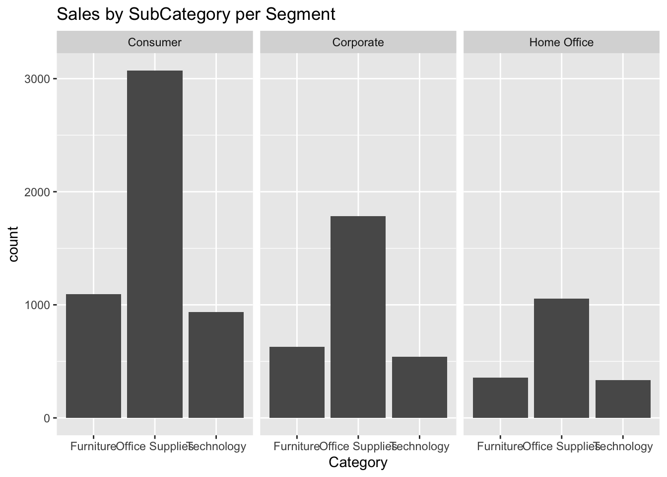
ggplot(data, aes(Segment)) +
geom_bar() +
labs(title = "Sales by Segment per SubCategory") +
facet_wrap(vars(SubCategory))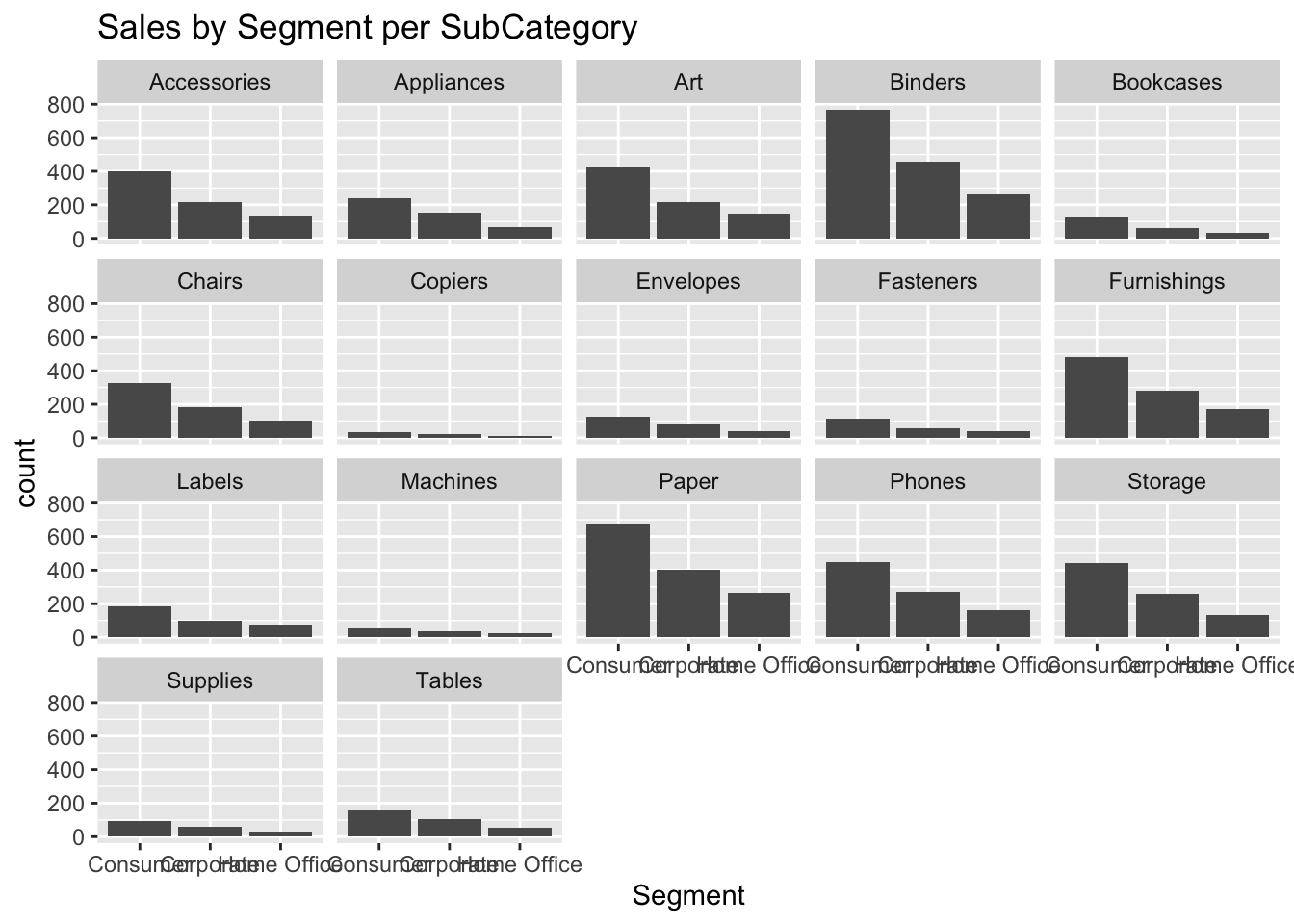
Explain why you choose to conduct these specific data analyses and visualizations. In other words, how do such types of statistics or graphs (see the R Gallery) help you answer specific questions? For example, how can a bivariate visualization reveal the relationship between two variables, or how does a linear graph of variables over time present the pattern of development?
If you plan to conduct specific data analyses and visualizations, describe how do you need to process and prepare the tidy data.
What do you need to do to mutate the datasets (convert date data, create a new variable, pivot the data format, etc.)?
How are you going to deal with the missing data/NAs and outliers? And why do you choose this way to deal with NAs?
(Optional) It is encouraged, but optional, to include a coding component of tidy data in this part.
totalSales <- newData %>%
group_by(Region) %>%
summarise(SalesTotal = sum(Sales)) %>%
select(Region, SalesTotal)
totalSalesggplot(totalSales, aes(Region, weight = SalesTotal)) +
geom_bar()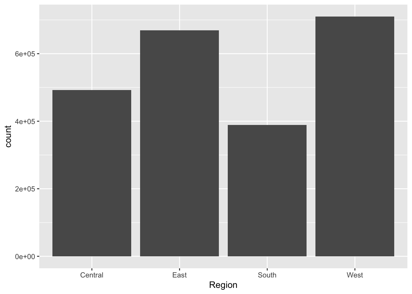
Special Note on the role of statistics
Statistical analyses are not required, but any students who wish to include these may do so. However, your primary analysis should center around visualization rather than inferential statistics. Many scientists only compute statistics after a careful process of exploratory data analysis and data visualization. Statistics are a way to gauge your certainty in your results - NOT A WAY TO DISCOVER MEANINGFUL DATA PATTERNS. Do not run a multiple regression with numerous predictors and report which predictors are significant!!
Remember: The goal is to tell a story about the data. For example, you might identify sports where winning athletes are younger or older than average and then try to see if you can find some sort of pattern that accounts for this difference. Or perhaps you might compare a country’s performance to GDP and see if this changes over time. The goal is not to get a significant statistical result but to identify an interesting pattern in the data and then extract some sort of meaningful recommendation or information from it.
Evaluation
You will be evaluated on both the quality of your source code and your written report, with a greater emphasis on the clarity and details of the description of your dataset(s) and your research questions.
model <- lm(Sales~Month+Year+Segment+Region+Category, data = newData)
print(model)
Call:
lm(formula = Sales ~ Month + Year + Segment + Region + Category,
data = newData)
Coefficients:
(Intercept) Month Year
12683.3511 -0.3413 -6.1223
SegmentCorporate SegmentHome Office RegionEast
8.3316 18.8295 19.5354
RegionSouth RegionWest CategoryOffice Supplies
27.0276 4.0789 -231.5232
CategoryTechnology
105.4207 cat("# # # # The Coefficient Values # # # ","\n")# # # # The Coefficient Values # # # a <- coef(model)[1]
print(a)(Intercept)
12683.35 XMonth <- coef(model)[2]
XYear <- coef(model)[3]
XYear <- coef(model)[4]
XSegmentHomeOffice<- coef(model)[5]
XRegionEast<- coef(model)[6]
XRegionSouth<- coef(model)[7]
XRegionWest<- coef(model)[8]
XCategoryOfficeSupplies<- coef(model)[9]
XCategoryOfficeSupplies<- coef(model)[10]
#predicting sales for year 2019 in the month of July for Corporate in Region East for Category Technology
X1 = 7
X2 = 2019
X3 = 1
X4 = 0
X5 = 1
X6 = 0
X7 = 0
X8 = 0
X9 = 1
Y = a + XMonth*X1 + XYear*X2 + XYear*X3 + XSegmentHomeOffice*X4 + XRegionEast*X5 + XRegionSouth*X6 + XRegionWest*X7 + XCategoryOfficeSupplies*X8 + XCategoryOfficeSupplies*X9
print(Y)(Intercept)
29635.8