Challenge 7

challenge_7

hotel_bookings

Visualizing Multiple Dimensions

Author

Pranav Komaravolu

Published

May 19, 2023

library(readr)
library(tidyverse)
library(ggplot2)
library(dplyr)
options(dplyr.summarise.inform = FALSE)

knitr::opts_chunk$set(echo = TRUE, warning=FALSE, message=FALSE)

Data Description

Reading the data

data <- read_csv("_data/hotel_bookings.csv", show_col_types = FALSE)
head(data)

# A tibble: 6 × 32
  hotel   is_ca…¹ lead_…² arriv…³ arriv…⁴ arriv…⁵ arriv…⁶ stays…⁷ stays…⁸ adults
  <chr>     <dbl>   <dbl>   <dbl> <chr>     <dbl>   <dbl>   <dbl>   <dbl>  <dbl>
1 Resort…       0     342    2015 July         27       1       0       0      2
2 Resort…       0     737    2015 July         27       1       0       0      2
3 Resort…       0       7    2015 July         27       1       0       1      1
4 Resort…       0      13    2015 July         27       1       0       1      1
5 Resort…       0      14    2015 July         27       1       0       2      2
6 Resort…       0      14    2015 July         27       1       0       2      2
# … with 22 more variables: children <dbl>, babies <dbl>, meal <chr>,
#   country <chr>, market_segment <chr>, distribution_channel <chr>,
#   is_repeated_guest <dbl>, previous_cancellations <dbl>,
#   previous_bookings_not_canceled <dbl>, reserved_room_type <chr>,
#   assigned_room_type <chr>, booking_changes <dbl>, deposit_type <chr>,
#   agent <chr>, company <chr>, days_in_waiting_list <dbl>,
#   customer_type <chr>, adr <dbl>, required_car_parking_spaces <dbl>, …

Columns in the dataset:

colnames(data)

 [1] "hotel"                          "is_canceled"                   
 [3] "lead_time"                      "arrival_date_year"             
 [5] "arrival_date_month"             "arrival_date_week_number"      
 [7] "arrival_date_day_of_month"      "stays_in_weekend_nights"       
 [9] "stays_in_week_nights"           "adults"                        
[11] "children"                       "babies"                        
[13] "meal"                           "country"                       
[15] "market_segment"                 "distribution_channel"          
[17] "is_repeated_guest"              "previous_cancellations"        
[19] "previous_bookings_not_canceled" "reserved_room_type"            
[21] "assigned_room_type"             "booking_changes"               
[23] "deposit_type"                   "agent"                         
[25] "company"                        "days_in_waiting_list"          
[27] "customer_type"                  "adr"                           
[29] "required_car_parking_spaces"    "total_of_special_requests"     
[31] "reservation_status"             "reservation_status_date"

The dimensions of the dataset are as follows:

dim(data)

[1] 119390     32

There are 32 columns and 119390 rows in the dataset.

Tidy Data (as needed)

I plan on visualizing the number of people who stayed in a hotel during each year so the dataset can be assumed to be tidy and can be used for visualization.

Visualization with Multiple Dimensions

First I want to analyse at which of these years the hotels had a maximum number of people staying at the hotel. To do that first I will have to filter out the people who cancelled from the dataset, then we can group the data on hotel and arrival_date_year and this data could be summarised to obtain the number of people staying in each of the hotels during different years. The command is as follows:

month_yearly_data <- data%>%
  filter(is_canceled == 0)%>%
  group_by(hotel, arrival_date_year, arrival_date_month)%>%
  mutate(total_people = adults + children + babies)%>%
  summarise(bookings = n(), total_guests = sum(total_people))

head(month_yearly_data)

# A tibble: 6 × 5
# Groups:   hotel, arrival_date_year [1]
  hotel      arrival_date_year arrival_date_month bookings total_guests
  <chr>                  <dbl> <chr>                 <int>        <dbl>
1 City Hotel              2015 August                 1248         2451
2 City Hotel              2015 December                986         1876
3 City Hotel              2015 July                    459          852
4 City Hotel              2015 November                934         1470
5 City Hotel              2015 October                2065         3634
6 City Hotel              2015 September              1986         3456

yearly_data <- month_yearly_data%>%
  group_by(hotel, arrival_date_year)%>%
  summarise(yearly_bookings = sum(bookings), yearly_guests = sum(total_guests))

head(yearly_data)

# A tibble: 6 × 4
# Groups:   hotel [2]
  hotel        arrival_date_year yearly_bookings yearly_guests
  <chr>                    <dbl>           <int>         <dbl>
1 City Hotel                2015            7678         13739
2 City Hotel                2016           22733         44433
3 City Hotel                2017           15817         31284
4 Resort Hotel              2015            6176         12205
5 Resort Hotel              2016           13637         26431
6 Resort Hotel              2017            9125         17915

Now we have a clear idea on the number of bookings that took place and the total number of guests that stayed in a hotel during a particular year. So now similar to the last experiment we try to plot a bar graph indicating these factors.

ggplot(yearly_data) + 
  geom_bar(aes(x = arrival_date_year, y = yearly_guests, fill = hotel), , stat = "identity", position = "dodge") +
  labs(title = "A bar graph depicting total number of guests every year")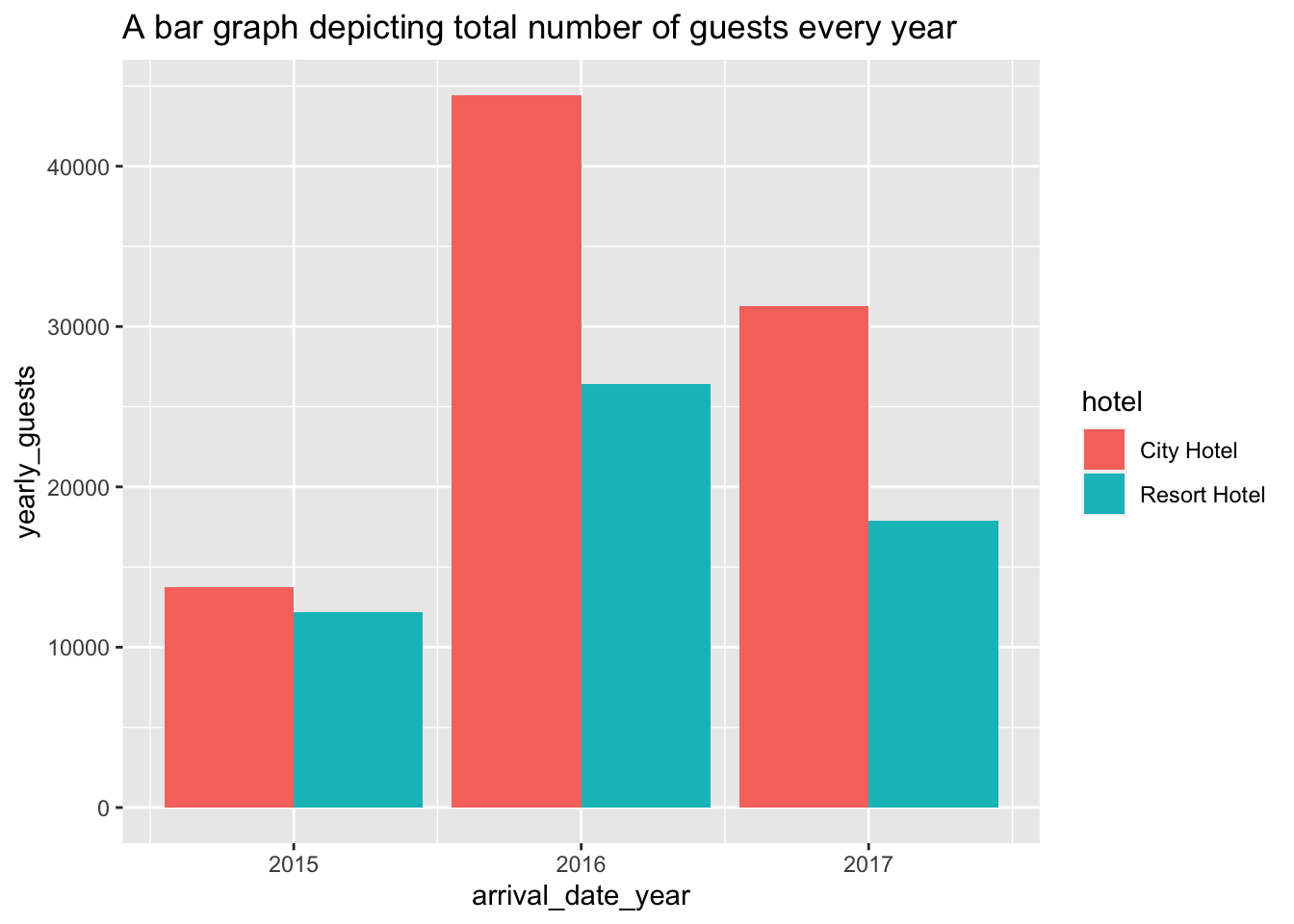

Now we need to visualize the third dimension i.e, months in which the number of guests were high. This information helps the hotel owners prepare well for any kind of future scenarios. We can visualize the three dimensions of yearly guests

ggplot(month_yearly_data, aes(x = arrival_date_year, y = total_guests, col = hotel)) +
  facet_wrap(vars(hotel))+
  geom_line() +
  geom_point()+
  geom_text(size=2.5, aes(label = arrival_date_month))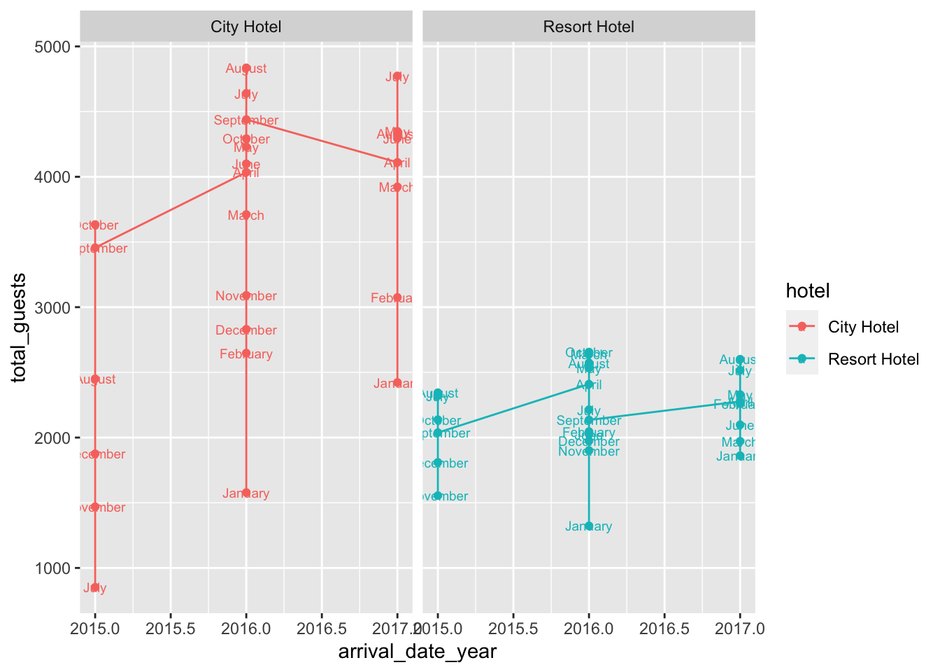

The above plot represents the number of guests that were present during each year and also depicts the number of guests each month.