Code
library(tidyverse)
knitr::opts_chunk$set(echo = TRUE, warning=FALSE, message=FALSE)
library(ggplot2)
library(readr)
library(openintro) #this is where the data set is hosted
library(leaps)
library(dplyr)
library(gridExtra)
library(flexmix)library(tidyverse)
knitr::opts_chunk$set(echo = TRUE, warning=FALSE, message=FALSE)
library(ggplot2)
library(readr)
library(openintro) #this is where the data set is hosted
library(leaps)
library(dplyr)
library(gridExtra)
library(flexmix)Understanding the effects of different variables on total selling price can help online vendors make decisions on how to list their products in order to sell them at the highest possible price point. I plan to examine what factors really impact the total selling price of Nintendo Wii Mario Kart games in Ebay auctions?
The data set I was working with from a website of data sets that were easily interchangeable with RStudio. Data is from 143 observations of Nintendo Wii Mario Kart auctions on Ebay that was collected October 2009. The data set has 12 descriptive variables composed of characteristics that are controlled by the seller ( e.g., starting price, condition of the item,duration of the auction) and response variables (e.g., number of bids, total price) for all auctions.
Dataset(s) Introduction:
The data set covers 143 observations of Ebay auctions made in one week. Auctions were included in the data set if they satisfied a series of conditions. Some factors were: if the auction did not end with a “Buy It Now” option, if the auction was listed in the Nintendo Wii section of Ebay, and if the item was being sold from the US etc. In my work I was most interested in which factors made for higher a total selling price of some auctions than others. After using the head function, I came to the conclusion that the variables that hold the most that the variables I am most interested in are duration (auction length in days), number of bids, condition (used/new), start price (USD) and total price. In future work I only use those variables of interest. I disregarded variables such as ID, number of wheels, and Title to strengthen and simplify my findings.
After using the head function I came to the conclusion that the variables that hold the most that the variables I am most interested in are duration (auction length in days), number of bids, condition (used/new), start price (USD) and total price. I disregarded variables such as ID, number of wheels, and Title to strengthen and simplify the findings.
ebay <- mariokart
dim(ebay)
[1] 143 12summary(ebay) id duration n_bids cond
Min. :1.104e+11 Min. : 1.000 Min. : 1.00 new :59
1st Qu.:1.404e+11 1st Qu.: 1.000 1st Qu.:10.00 used:84
Median :2.205e+11 Median : 3.000 Median :14.00
Mean :2.235e+11 Mean : 3.769 Mean :13.54
3rd Qu.:2.954e+11 3rd Qu.: 7.000 3rd Qu.:17.00
Max. :4.001e+11 Max. :10.000 Max. :29.00
start_pr ship_pr total_pr ship_sp
Min. : 0.010 Min. : 0.000 Min. : 28.98 standard :33
1st Qu.: 0.990 1st Qu.: 0.000 1st Qu.: 41.17 upsGround :31
Median : 1.000 Median : 3.000 Median : 46.50 priority :23
Mean : 8.777 Mean : 3.144 Mean : 49.88 firstClass:22
3rd Qu.:10.000 3rd Qu.: 4.000 3rd Qu.: 53.99 parcel :16
Max. :69.950 Max. :25.510 Max. :326.51 media :14
(Other) : 4
seller_rate stock_photo wheels
Min. : 0 no : 38 Min. :0.000
1st Qu.: 109 yes:105 1st Qu.:0.000
Median : 820 Median :1.000
Mean : 15898 Mean :1.147
3rd Qu.: 4858 3rd Qu.:2.000
Max. :270144 Max. :4.000
title
BRAND NEW NINTENDO MARIO KART WITH 2 WHEELS :23
Mario Kart Wii (Wii) :19
BRAND NEW NINTENDO 1 WII MARIO KART WITH 2 WHEELS +GAME: 8
Mario Kart Wii (GAME ONLY/NO WHEEL) - Nintendo Wii Game: 4
Mario Kart Wii (Wii) Nintendo Wii game *--WOW --AWESOME: 4
(Other) :84
NA's : 1 head(ebay %>% select(duration, n_bids, cond, start_pr, seller_rate, stock_photo, total_pr))The case of this data set is an individual auction of a Mario Kart Wii game represented by each row in the data set. The data set is composed of characteristics that are controlled by the seller ( e.g., starting price, condition of the item,duration of the auction) and response variables (e.g., number of bids, total price) for all auctions (143).
Through calculating summary statistics of my variables of interest, what stood out the most was total price. The maximum total price was 326.51 dollars which was more than 5 times the highest starting price. This was odd to because the mean total price was 49.88 dollars. The substantial jump in total price level interested me to look further into the category.
#Try gallery of plots
library(GGally)
ggpairs(ebay %>% select(duration, n_bids, cond, start_pr, seller_rate, stock_photo, total_pr))+
  theme_bw()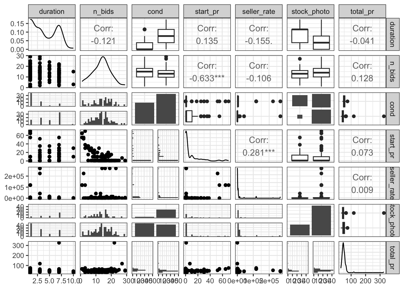
fit_full <- lm(total_pr ~ duration + start_pr + cond + stock_photo + seller_rate + n_bids, data = ebay)

ebay <- ebay %>%
  mutate(
    resid = residuals(fit_full)
  )
p1 <- ggplot(data = ebay, mapping = aes(x = duration, y = resid)) +
  geom_point() +
  geom_smooth() +
  theme_bw()
p2 <- ggplot(data = ebay, mapping = aes(x = start_pr, y = resid)) +
  geom_point() +
  geom_smooth() +
  theme_bw()
p3 <- ggplot(data = ebay, mapping = aes(x = cond, y = resid)) +
  geom_point() +
  geom_smooth() +
  theme_bw()
p4 <- ggplot(data = ebay, mapping = aes(x = stock_photo, y = resid)) +
  geom_point() +
  geom_smooth() +
  theme_bw()
p5 <- ggplot(data = ebay, mapping = aes(x = seller_rate, y = resid)) +
  geom_point() +
  geom_smooth() +
  theme_bw()
p6 <- ggplot(data = ebay, mapping = aes(x = n_bids, y = resid)) +
  geom_point() +
  geom_smooth() +
  theme_bw()
p7 <- ggplot(data = ebay, mapping = aes(x = resid)) +
  geom_density() +
  theme_bw()
grid.arrange(p1, p2, p3, p4, p5, p6, p7)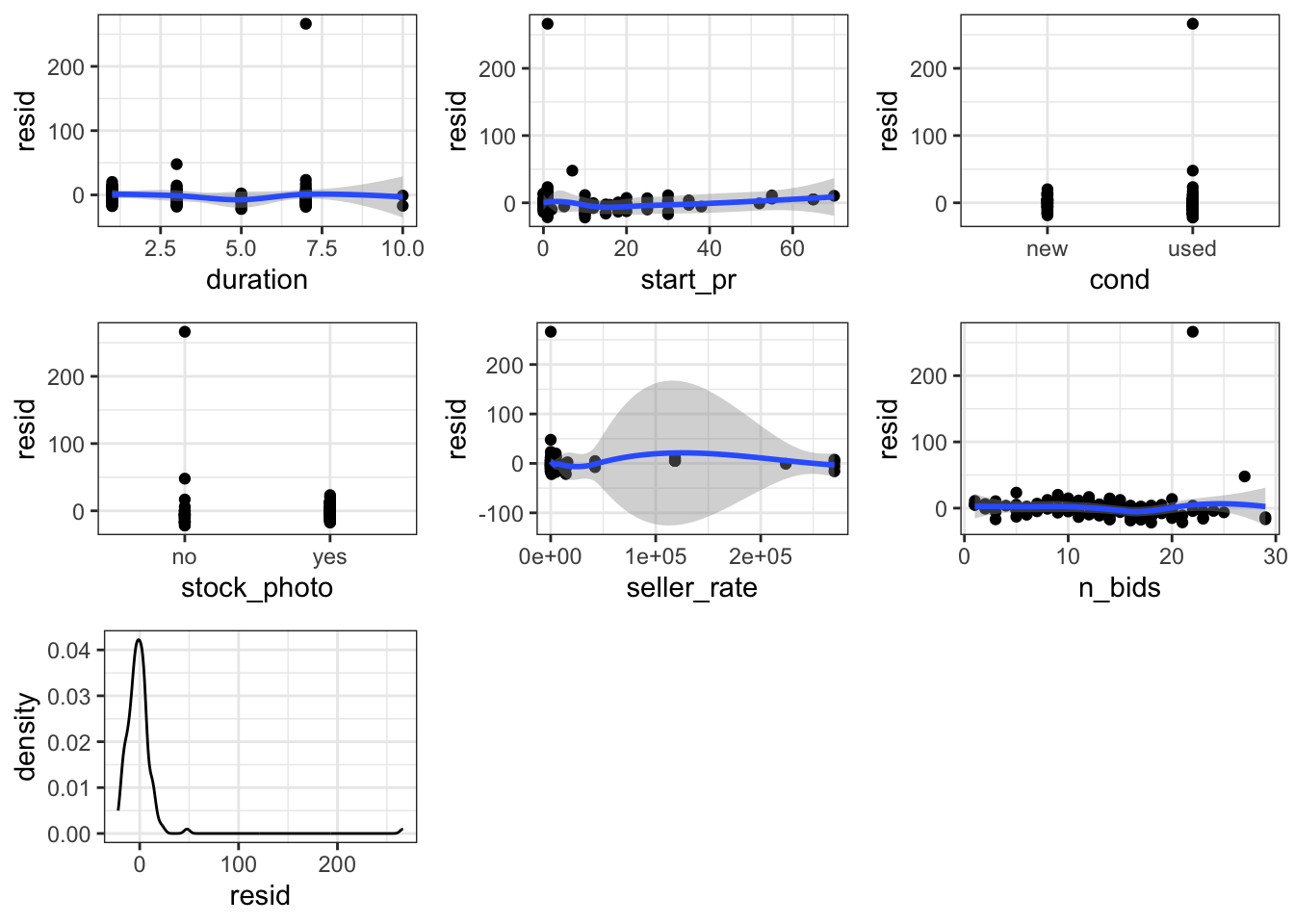
When using the GGpair function I can build a large matrix of plots that is much easier to visualize the distribution and correlations between variables of interest. In writing my code I chose to focus on my variables of interest I had previously set up. The chart shows fairly insignificant levels of correlation between starting price and duration of the bid, but a significant level of correlation between the starting price and the number of bids.
Within the GGpair graphs we see the presence of outliers and when looking through the data set there are two apparent outliers. Both outliers have total price levels above 80 dolalrs but no other discernible differences across the other variables. The unexplainable jump in total price led me to believe I should apply a transformation of the variables or just remove those two data points for clarity.
I wanted to use a regression later on to determine the level of influence of each variable upon total price, but first I needed to check if the regression conditions were met. I created diagnostic plots of the residuals of auction duration, starting price, condition of the listing, whether the listing had a photo, seller rate, the number of bids. The results showed that most regression conditions were not met (no normality, multiple outliers, unequal standars deviations). I will discuss the particularly unequal standard deviations of seller rate later, but the wide bin of the distribution of residuals immediately stood out as an area of concern.Based on the initial plots it was difficult to see notable significance because of the outliers so I went on to apply a logarithmic transformation (log of seller rate and log of total price), and manually remove the outliers. I applied transformations to those two and then was able to assume the conditions of linear regression are met and move on with further visualization and analysis.
I chose to apply a log transformation to seller rate and total price as seller rate in attempts to normalize the results. As I mentioned earlier from mapping residuals, seller rate was a factor that had an incredibly wide spread distribution. The mean seller rate was 15898.42 meaning that the average seller rate had 15898.42 positive ratings. The wide spread distribution (shown by the gray bin of the residual graph) comes from the standard deviation of 51840.32 positive reviews. The very high standard deviation meas that there is an incredibly wide spread of data and indicates that a transformation may be a useful tool to normalize the results.Pre-transformation, the data was too cluttered and confusing for clear conclusions to be reached. Post transformation the skewed original data is much more normal. It improved linearity between seller rate and total price as seen in the now significant correlation between total price and duration.
Although the analyses post transformation was much stronger for regression, it still seemed like there were outliers that were skewing the results and so I decided to manually remove the outliers. In order to identify what the outliers exactly were and the influence of them I ran a test of Cooks Distance and Hat Values.
ebay_transformed <- ebay_transformed %>%
  mutate(
    obs_index = row_number(),
    h = hatvalues(fit_full),
    D = cooks.distance(fit_full)
  )


ggplot(data = ebay_transformed, mapping = aes(x = obs_index, y = h)) +
  geom_hline(yintercept = 2 * 7 / nrow(ebay_transformed))+
  geom_point() +
  theme_bw()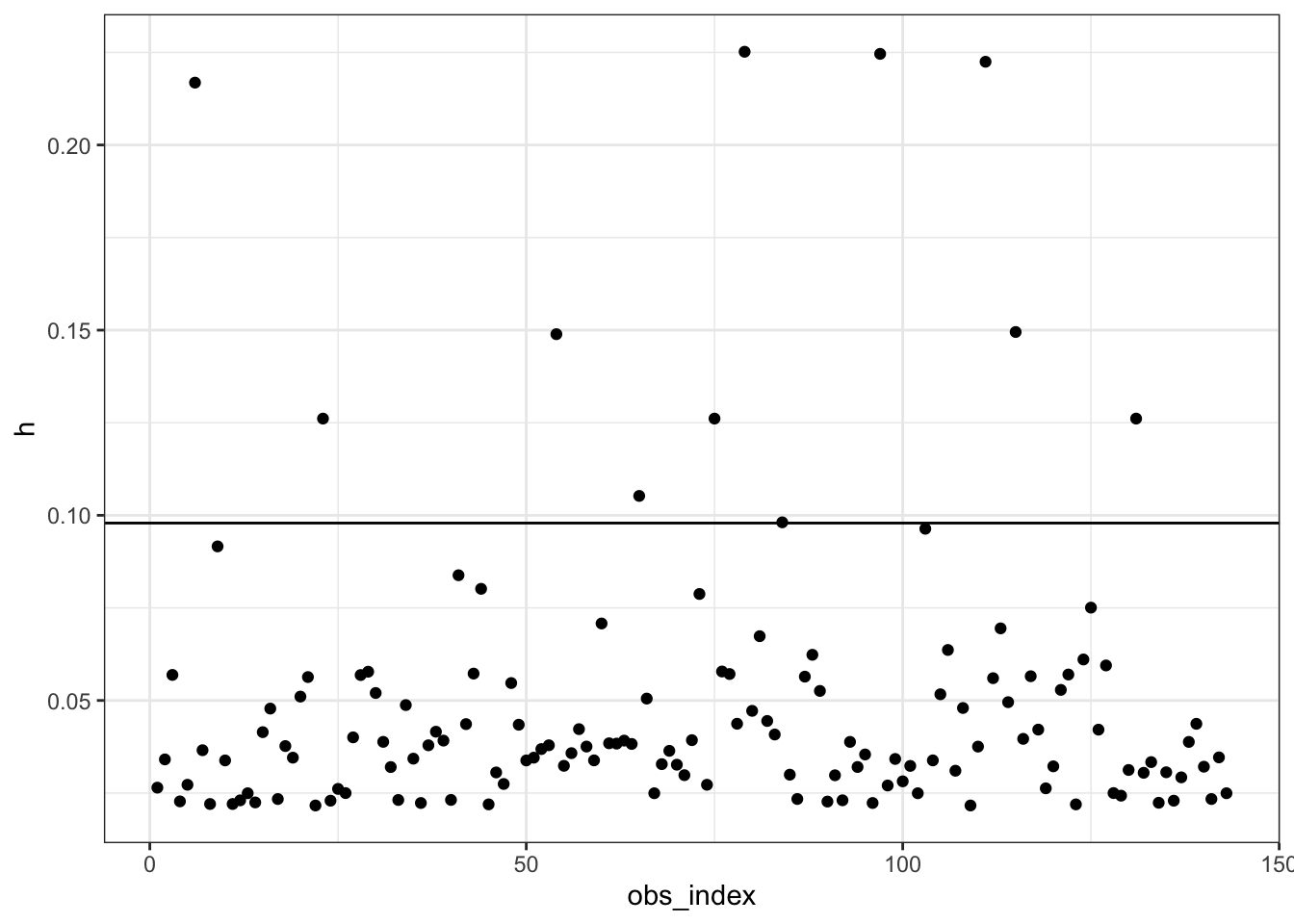
ggplot(data = ebay_transformed, mapping = aes(x = obs_index, y = D)) +
  geom_point() +
  theme_bw()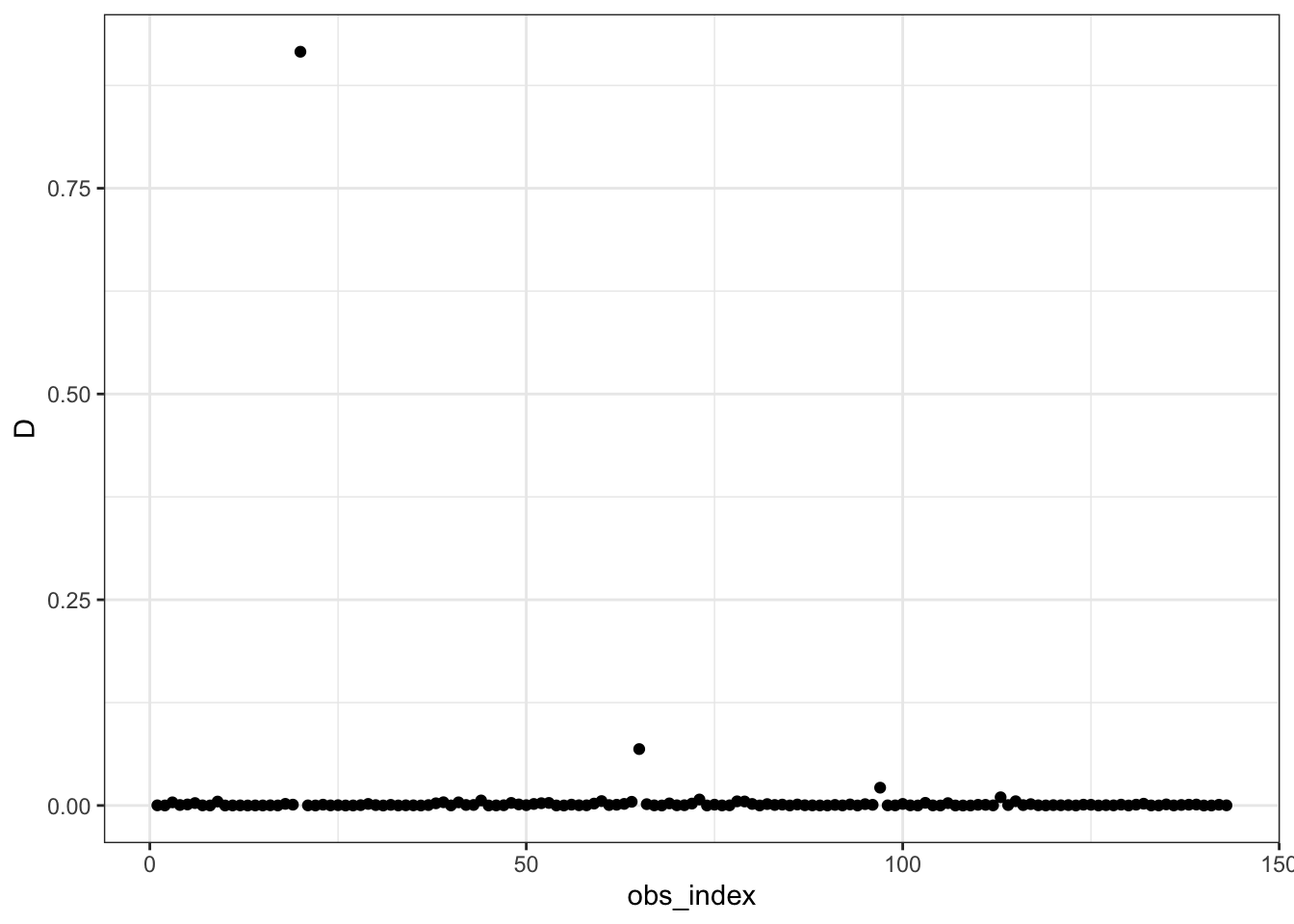
The Cooks Distance test outlined two clear areas of influence that were negatively impacting the relationship of the data and a possible regression I may want to run. The two clear suspicions exist at the observation index of 20 and 65, so from here on out I made sure to manually remove them. I also used Hat Values to double check for outliers by measuring how distant a point it from its’ corresponding ‘fitted point’. The Hat Values indicated possible outliers at values 9, 20, 23, 65, 75, 84, 103, 115, and 131. I use this information to manually remove these points of concern (hereafter referred to as “suspicions”).
ebay_transformed <- ebay_transformed %>%
  mutate(suspicious1 = obs_index %in% c(20, 65),
         suspicious2 = obs_index %in% c(9, 20, 23, 65, 75, 84, 103, 115, 131))

ggpairs(ebay_transformed %>% filter(!suspicious1) %>% select(duration, n_bids, cond, start_pr, log_seller_rate, stock_photo, log_total_pr))+
  theme_bw()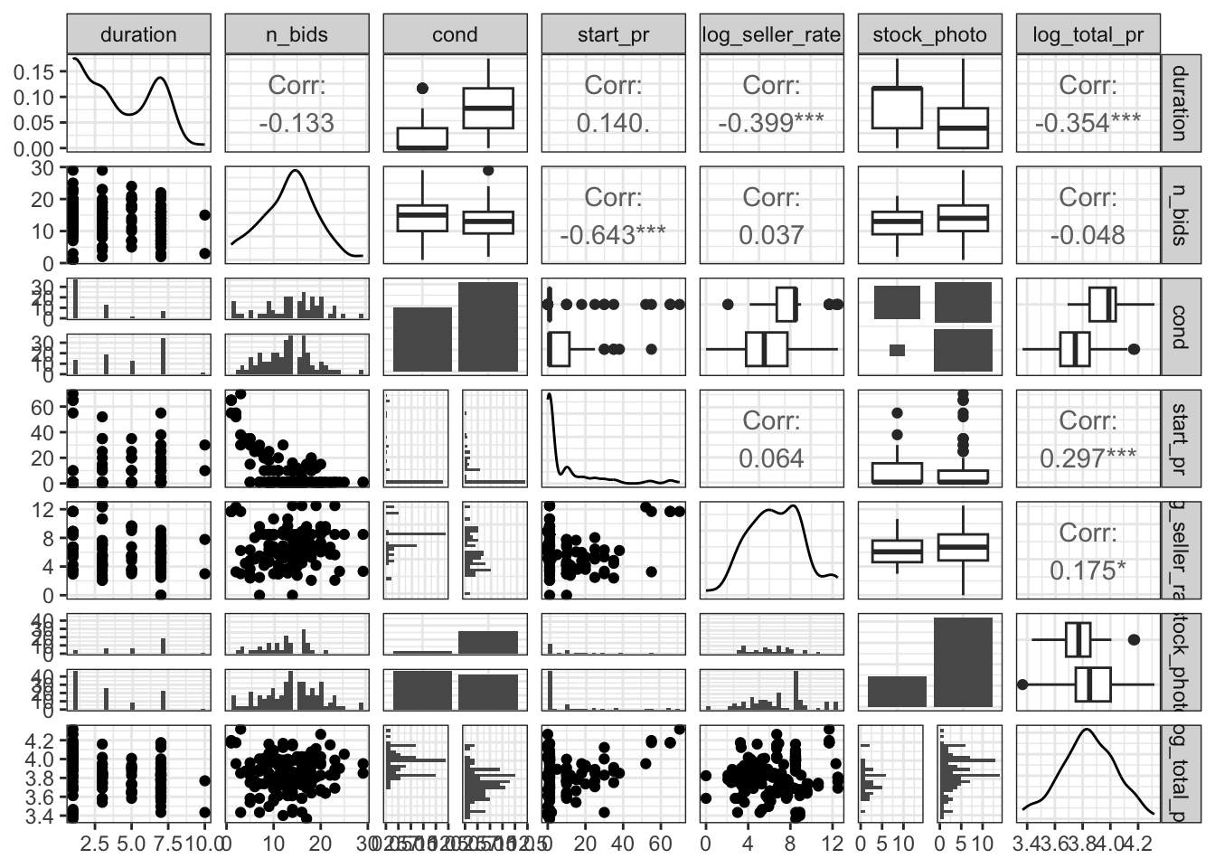
ggpairs(ebay_transformed %>% filter(!suspicious2) %>% select(duration, n_bids, cond, start_pr, log_seller_rate, stock_photo, log_total_pr))+
  theme_bw()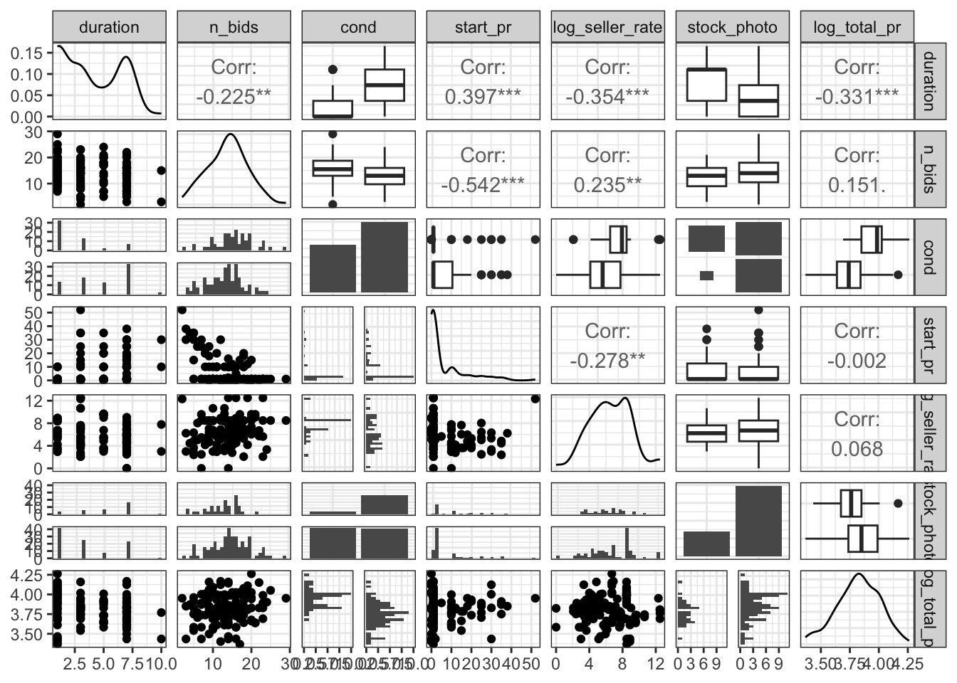
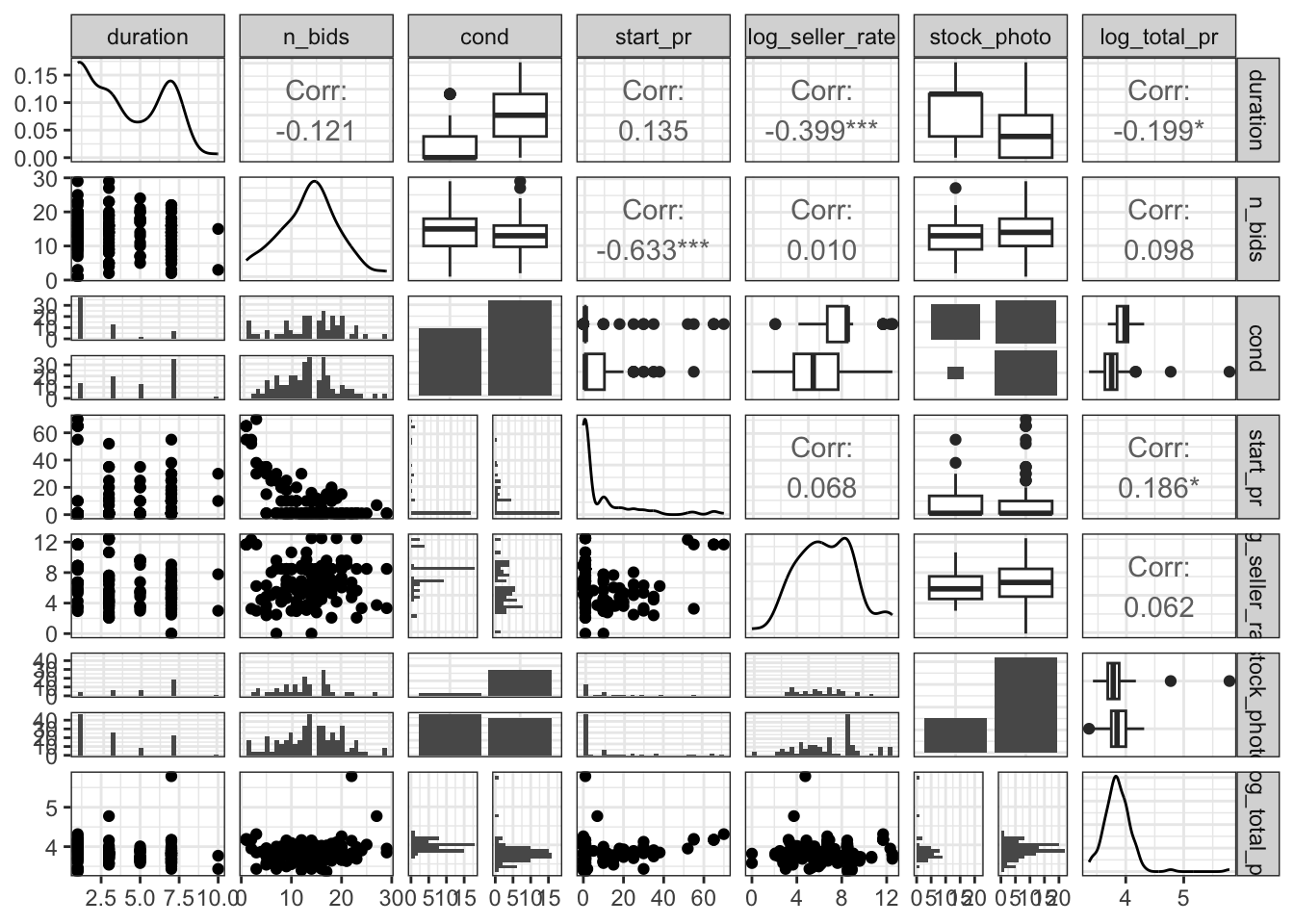
To get a final visualization of the effects of log total price upon my variables of interest I ran the ggpairs function again. This time there is much stronger significance between log total price and most other variables. The most significant correlation is between log total price and duration of the auction. There is a -0.354 correlation between log total price and duration of the auction. Meaning that as log total price increases the duration of the auction decreases significantly. Similarly to duration, there is a higher significance in starting price and log total price than before. After removing the Suspicious 2 (those found with the Hat Values method) there is a 0.297 correlation between starting price and log total price. Meaning that 29.7% of the variation between log total price of the auctions can be explained by the starting price of the auction. Although ordinarily a correlation coefficient(r-value) of 0.297 may be regarded as weak, the relationship was deemed a significant at the 0.05 level. When we compare this r-value to others for log total price, no other variable has as strong of a correlation. Take log seller rate for example, there is a 0.175 correlation between log total price and log seller rate. This light level of correlation means that 17.5 of the variation between log total price of the auctions can be explained by the log seller rate. After accounting for duration and start price, there was not significant evidence for a relationship between the other explanatory variables and total price. Based on the above ggpairs plot and correlation coefficients, it seems that there is the strong evidence of a positive association between total price, and start price, with a moderate negative association between duration and total price.
In order to run a regression I want to be sure I am selecting the strongest model for regression.I ran each regressions BIC individually to avoid confusion and began with Model 1 (full model)
#First Model
lm_fit_1 <- lm(log_total_pr ~ duration + start_pr + cond + stock_photo + log_seller_rate + n_bids, data = ebay_transformed)
summary(lm_fit_1)
Call:
lm(formula = log_total_pr ~ duration + start_pr + cond + stock_photo +
    log_seller_rate + n_bids, data = ebay_transformed)

Residuals:
     Min       1Q   Median       3Q      Max
-0.39974 -0.11510 -0.00051  0.08708  1.88640

Coefficients:
                 Estimate Std. Error t value Pr(>|t|)
(Intercept)      3.959438   0.116114  34.099  < 2e-16 ***
duration        -0.016454   0.009343  -1.761  0.08047 .
start_pr         0.006848   0.001707   4.012 9.88e-05 ***
condused        -0.194347   0.048005  -4.048 8.61e-05 ***
stock_photoyes  -0.110287   0.048633  -2.268  0.02492 *
log_seller_rate -0.014117   0.008315  -1.698  0.09186 .
n_bids           0.014200   0.004311   3.294  0.00126 **
---
Signif. codes:  0 '***' 0.001 '**' 0.01 '*' 0.05 '.' 0.1 ' ' 1

Residual standard error: 0.231 on 136 degrees of freedom
Multiple R-squared:  0.2603,    Adjusted R-squared:  0.2277
F-statistic: 7.976 on 6 and 136 DF, p-value: 2.215e-07#Plot the candidates models
candidate_models1 <- regsubsets(log_total_pr ~ duration + start_pr + cond + stock_photo + log_seller_rate + n_bids, data = ebay_transformed)
plot(candidate_models1)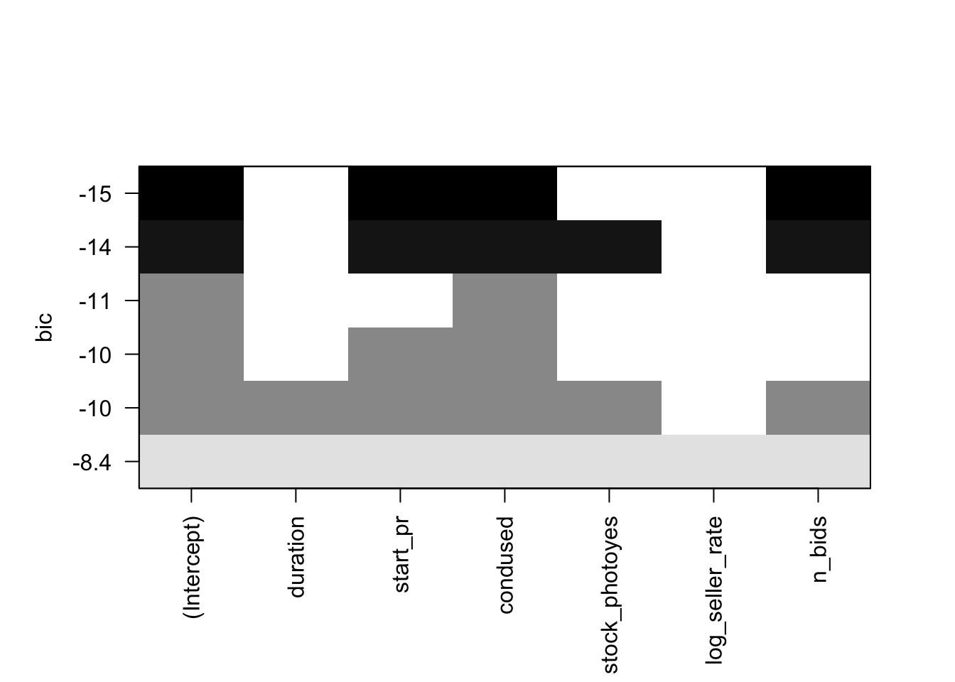
I used the BIC metric to compare best fit for each of the models. Model 1 (the full model with no outliers removed) had the largest BIC value of 19.22. This is our model with all variables we want to check on the transformed scale. It indicates that adding variables “condused”, “log_total_price” and “start_pr” will likely be of value. Interestingly, it is the only model where n_bids is significant, however I disregard the full model as it has a very high BIC which is indicative of a poor fit, and chose to move forward with the second model
#Filter out major outliers - 2 different subsets
lm_fit_2 <- lm(log_total_pr ~ duration + start_pr + cond + stock_photo + log_seller_rate + n_bids, data = ebay_transformed %>% filter(!suspicious1))
summary(lm_fit_2)
Call:
lm(formula = log_total_pr ~ duration + start_pr + cond + stock_photo +
    log_seller_rate + n_bids, data = ebay_transformed %>% filter(!suspicious1))

Residuals:
     Min       1Q   Median       3Q      Max
-0.38403 -0.09451  0.01179  0.08768  0.48784

Coefficients:
                 Estimate Std. Error t value Pr(>|t|)
(Intercept)      3.997082   0.072485  55.143  < 2e-16 ***
duration        -0.015715   0.005893  -2.667   0.0086 **
start_pr         0.005004   0.001085   4.610 9.27e-06 ***
condused        -0.206214   0.030015  -6.870 2.19e-10 ***
stock_photoyes  -0.030930   0.031016  -0.997   0.3205
log_seller_rate -0.009011   0.005226  -1.724   0.0870 .
n_bids           0.004599   0.002825   1.628   0.1059
---
Signif. codes:  0 '***' 0.001 '**' 0.01 '*' 0.05 '.' 0.1 ' ' 1

Residual standard error: 0.1441 on 134 degrees of freedom
Multiple R-squared:  0.4651,    Adjusted R-squared:  0.4412
F-statistic: 19.42 on 6 and 134 DF, p-value: 3.257e-16p1 <- ggplot(data = ebay_transformed %>% filter(!suspicious1), mapping = aes(x = duration, y = resid)) +
geom_point() +
geom_smooth() +
theme_bw()
p2 <- ggplot(data = ebay_transformed %>% filter(!suspicious1), mapping = aes(x = start_pr, y = resid)) +
geom_point() +
geom_smooth() +
theme_bw()
p3 <- ggplot(data = ebay_transformed %>% filter(!suspicious1), mapping = aes(x = cond, y = resid)) +
geom_point() +
geom_smooth() +
theme_bw()
p4 <- ggplot(data = ebay_transformed %>% filter(!suspicious1), mapping = aes(x = stock_photo, y = resid)) +
geom_point() +
geom_smooth() +
theme_bw()
p5 <- ggplot(data = ebay_transformed %>% filter(!suspicious1), mapping = aes(x = log_seller_rate, y = resid)) +
geom_point() +
geom_smooth() +
theme_bw()
p6 <- ggplot(data = ebay_transformed %>% filter(!suspicious1), mapping = aes(x = n_bids, y = resid)) +
geom_point() +
geom_smooth() +
theme_bw()
p7 <- ggplot(data = ebay_transformed %>% filter(!suspicious1), mapping = aes(x = resid)) +
geom_density() +
theme_bw()
grid.arrange(p1, p2, p3, p4, p5, p6, p7)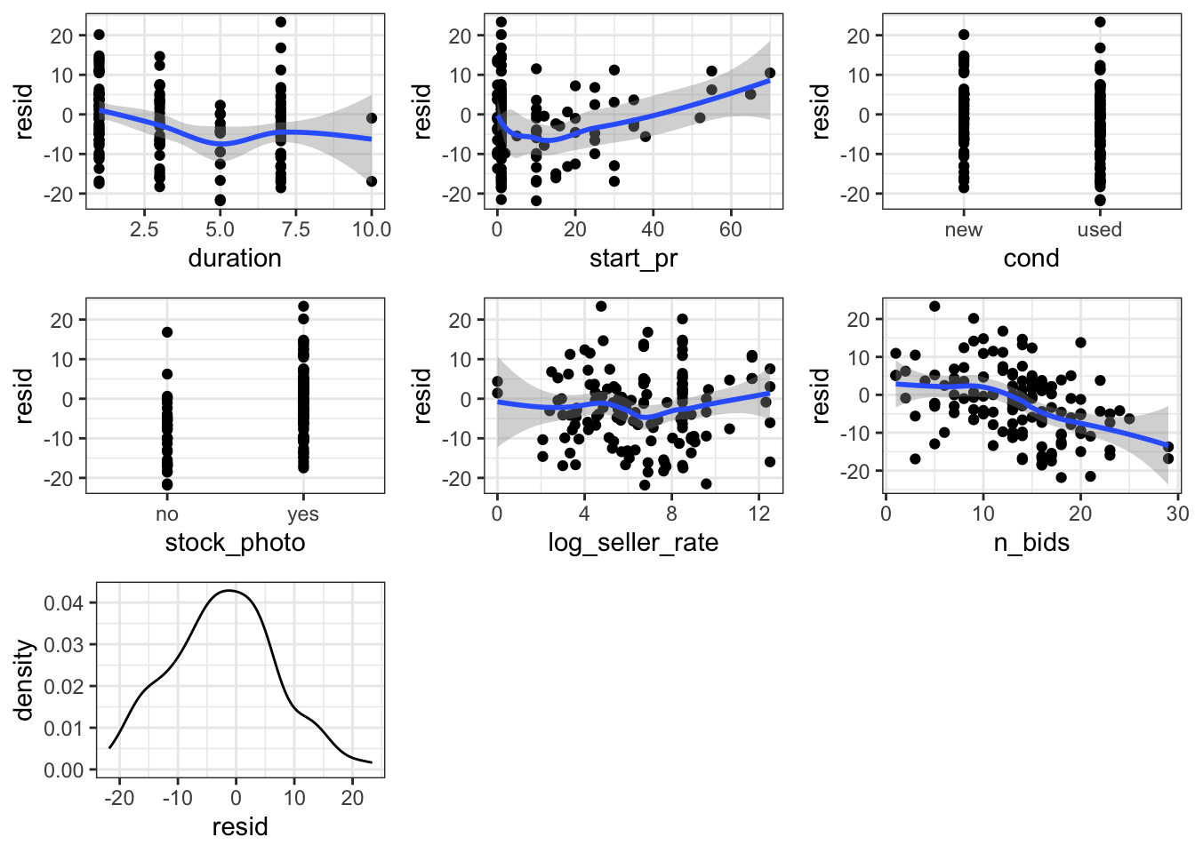
candidate_models2 <- regsubsets(log_total_pr ~ duration + start_pr + cond + stock_photo + log_seller_rate + n_bids, data = ebay_transformed %>% filter(!suspicious1))
plot(candidate_models2)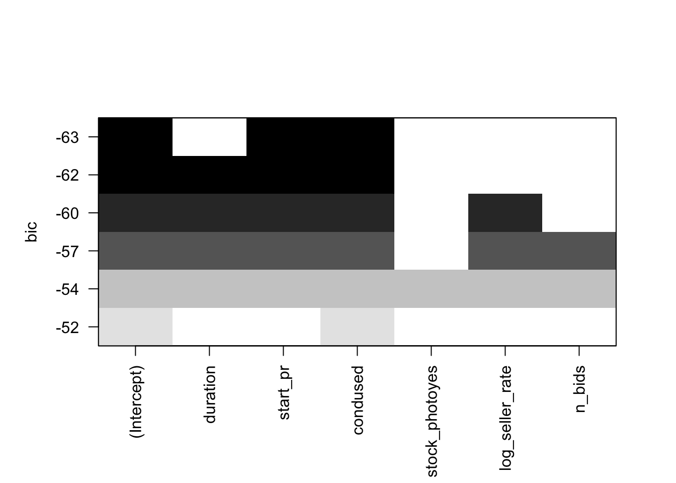
I repeated the BIC process from above for Model 2 (model with 2 suspicious removed). Similar to the model before, this BIC indicates that the most impactful variables for the regression are “condused”, “totalprice”, “duration” and “startpr”. The BIC shows start price and condition to be most significant. Duration and bids were also significant, but to a lesser extent. N_Bids was only significant before the removal of outliers, but Stock photo and seller rate were not significant across either model.
lm_fit_2 <- lm(log_total_pr ~ duration + start_pr + cond + stock_photo + log_seller_rate + n_bids, data = ebay_transformed %>% filter(!suspicious1))
summary(lm_fit_2)
Call:
lm(formula = log_total_pr ~ duration + start_pr + cond + stock_photo +
    log_seller_rate + n_bids, data = ebay_transformed %>% filter(!suspicious1))

Residuals:
     Min       1Q   Median       3Q      Max
-0.38403 -0.09451  0.01179  0.08768  0.48784

Coefficients:
                 Estimate Std. Error t value Pr(>|t|)
(Intercept)      3.997082   0.072485  55.143  < 2e-16 ***
duration        -0.015715   0.005893  -2.667   0.0086 **
start_pr         0.005004   0.001085   4.610 9.27e-06 ***
condused        -0.206214   0.030015  -6.870 2.19e-10 ***
stock_photoyes  -0.030930   0.031016  -0.997   0.3205
log_seller_rate -0.009011   0.005226  -1.724   0.0870 .
n_bids           0.004599   0.002825   1.628   0.1059
---
Signif. codes:  0 '***' 0.001 '**' 0.01 '*' 0.05 '.' 0.1 ' ' 1

Residual standard error: 0.1441 on 134 degrees of freedom
Multiple R-squared:  0.4651,    Adjusted R-squared:  0.4412
F-statistic: 19.42 on 6 and 134 DF, p-value: 3.257e-16I ran a linear regression of Model 2(model with two suspicions removed). I used the results of the regression to create the following model statement:
\(μ(log(price)| duration,startprice,condition)=3.997-0.16duration +0.005startpr - 0.206condition\)
Without any other factors, the total price of a Mario Kart Wii auction on ebay is 3.997 dollars, however in the case of this problem the intercept does not necessarily make sense. It is not possible to sell an item on ebay without it having it meet some (if not all) of the other qualifications/variables. For every one day increase in auction duration, total price of Mario Kart Wii auction decreases by .16 dollars. If start price increases by one dollar, total price increases by 0.005. Finally, if the condition of the game was used the total price of the auction was 0.206 dollars lower.The two outliers model (chosen model) had a p-value = < 2e-16 and 95% CI: (3.854, 4.140). In other words, there is 95% confidence the intercept for log_total_price is between 3.854 and 4.140 (log) dollars.
I’ve never really used R-studio before, so I wanted to select a data set that would keep me interested and engaged with the material. I have friends who are depop/ebay sellers who thrift goods and then resell them and wanted to gain insight in what effects selling price. The data set was made of 143 observations of Ebay auctions made in one week. I initially focused on the following variables: duration (auction length in days), number of bids, condition (used/new), start price (USD) and total price. Towards the end of my work my variables of interest changed, and I did so using BIC modeling. I shifted my focus to duration of auction, starting price and condition of item.
I began by mutating the data by applying a log transformation of the total price and seller rate which removed some skew and outliers but not all. I realized I had to do further work in modifying the data set so I worked to manually remove the data points. I created a full model (had no removal of outliers) and a second model (removed two suspicions) that allowed me to come to stronger and more accurate conclusions.
All of the models with the low BIC showed strong evidence of a positive association between total price, and start price, and the models with outliers removed showed moderate negative association between duration and total price (contradicting the literature), among listings similar to those in this study. The results were most significant when only the two outliers were removed, followed by multiple suspicious values being removed, and the full model showed the weakest significance. Regardless, after accounting for duration and start price, there was not significant evidence for a relationship between the other explanatory variables and total price.
The data contains a large proportion of outliers, so if I were to conduct the project again, I might look for another data set with a larger sample to help normalize the data set. I believe manually removing the outliers helped remove skew the data set and allow for me to run a regression later. It is possible that because the survey was conducted closely after the game released, demand for the game may have altered total price. If we were the designers, we might want to expand the sample selection to include other driving games released at a similar time. It is possible that factors like popularity impacted the final selling prices across games. For example, if “Mario Kart Wii” had different total price than “Asphalt:4” (a similar game introduced at the same time) we might assume demand for a game impacts total price. By only focusing on one game, we do not control for omitted variable bias and possible interaction between the variables.
Data set: R: Wii Mario Kart auctions from Ebay https://vincentarelbundock.github.io/Rdatasets/articles/data.html
R Packages: library(ggplot2) library(readr) library(openintro) library(leaps) library(dplyr) library(GGally)
Literature: Ariely, D., & Simonson, I. (2003). Buying, bidding, playing, or competing? value assessment and decision dynamics in online auctions. Journal of Consumer Psychology, 13(1), 113–123. https://doi.org/10.1207/153276603768344834
The R Graph Gallery- https://r-graph-gallery.com/
Wickham, H., & Grolemund, G. (2016). R for data science: Visualize, model, transform, tidy, and import data. OReilly Media.
Feng, Changyong, et al. “Log-Transformation and Its Implications for Data Analysis.” Shanghai Archives of Psychiatry, Apr. 2014, www.ncbi.nlm.nih.gov/pmc/articles/PMC4120293/#:~:text=The%20log%20transformation%20is%2C%20arguably,normal%20or%20near%20normal%20distribution