Introduction

I was trying to analyze the ‘wild_bird_data.xlsx’ dataset in order to determine the subject of the dataset. This dataset summarizes the population size of wild bird species based on their body weight. We first start by importing the necessary libraries and setting the working directory to point to the location where the spreadsheet is located.

Code

library(tidyverse)
library(readxl)
library(ggplot2)
knitr::opts_chunk$set(echo = TRUE, warning=FALSE, message=FALSE)
setwd("D:/MyDocs/Class Slides/DACSS601/601_Spring_2023/posts/_data")

Clean file and Obtain Summary Statistics

Notice that the first line in the spreadsheet is referring to where data is obtained from. This line is removed and the data is summarized for both the columns.Notice that the mean is a lot lesser than the maximum value for both the columns indicating that there are some very large value outliers in the dataset. The data is also left skewed as there are a lot of values clustered around the left. The mean is higher than the median because the few outliers pull the mean up.

Code

setwd("D:/MyDocs/Class Slides/DACSS601/601_Spring_2023/posts/_data")
dataframe <- read_excel("wild_bird_data.xlsx", skip=1)
print(dataframe)

# A tibble: 146 × 2
   `Wet body weight [g]` `Population size`
                   <dbl>             <dbl>
 1                  5.46           532194.
 2                  7.76          3165107.
 3                  8.64          2592997.
 4                 10.7           3524193.
 5                  7.42           389806.
 6                  9.12           604766.
 7                  8.04           192361.
 8                  8.70           250452.
 9                  8.89            16997.
10                  9.52              595.
# … with 136 more rows

Code

summary(dataframe$`Population size`)

   Min. 1st Qu.  Median    Mean 3rd Qu.    Max. 
      5    1821   24353  382874  198515 5093378 

Code

summary(dataframe$`Wet body weight [g]`)

    Min.  1st Qu.   Median     Mean  3rd Qu.     Max. 
   5.459   18.620   69.232  363.694  309.826 9639.845 

Decribe data

First sorted the data according to the individual body weight and then assign each to a WeightClass in order to understand which category each bird falls into. Also assigned each bird to a PopulationClass based on Population Size. Plotted graphs which further confirm the skewness.

Code

dataframe <- arrange(dataframe, `Wet body weight [g]`)
dataframe <- mutate(dataframe, WtClass = case_when(
  `Wet body weight [g]` <= 10 ~ "Flyweight",
  `Wet body weight [g]` > 10 & `Wet body weight [g]` <= 30 ~ "Bantamweight",
  `Wet body weight [g]` > 30 & `Wet body weight [g]` <= 60 ~ "Featherweight",
  `Wet body weight [g]` > 60 & `Wet body weight [g]` <= 100 ~ "Lightweight",
  `Wet body weight [g]` > 100 & `Wet body weight [g]` <= 300 ~ "Welterweight",
  `Wet body weight [g]` > 300 & `Wet body weight [g]` <= 600 ~ "Middleweight",
  `Wet body weight [g]` > 600 & `Wet body weight [g]` <= 1000 ~ "Light HeavyWeight",
  `Wet body weight [g]` > 1000 ~ "Heavyweight"
))

dataframe <- mutate(dataframe, PopulationClass = case_when(
  `Population size` <= 1000000 ~ "< 1M",
  `Population size` > 1000000 & `Population size` <= 2000000 ~ "1M-2M",
  `Population size` > 2000000 & `Population size` <= 3000000 ~ "2M-3M",
  `Population size` > 3000000 & `Population size` <= 4000000 ~ "3M-4M",
  `Population size` > 4000000 & `Population size` <= 5000000 ~ "4M-5M",
  `Population size` > 5000000 ~ "> 5M",
))
print(dataframe)

# A tibble: 146 × 4
   `Wet body weight [g]` `Population size` WtClass      PopulationClass
                   <dbl>             <dbl> <chr>        <chr>          
 1                  5.46           532194. Flyweight    < 1M           
 2                  7.42           389806. Flyweight    < 1M           
 3                  7.76          3165107. Flyweight    3M-4M          
 4                  8.04           192361. Flyweight    < 1M           
 5                  8.64          2592997. Flyweight    2M-3M          
 6                  8.70           250452. Flyweight    < 1M           
 7                  8.89            16997. Flyweight    < 1M           
 8                  9.12           604766. Flyweight    < 1M           
 9                  9.52              595. Flyweight    < 1M           
10                 10.1             74386. Bantamweight < 1M           
# … with 136 more rows

Code

ggplot(dataframe, aes(`WtClass`)) + geom_bar()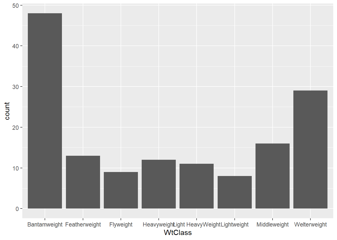

Code

ggplot(dataframe, aes(`PopulationClass`)) + geom_bar()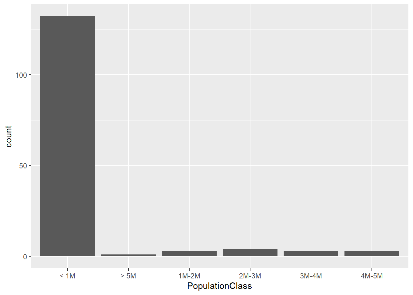

Conclusion

The wild_bird_data.xlsx contains information about wild bird species based on individual body weight and Population size