Code
library(tidyverse)
library(readxl)
library(DescTools)
knitr::opts_chunk$set(echo = TRUE, warning=FALSE, message=FALSE)
setwd("D:/MyDocs/Class Slides/DACSS601/601_Spring_2023/posts/_data")I was trying to analyze the ‘birds.csv’ dataset by splitting the data into different subgroups in order to interpret the meaning of the results. This dataset summarizes the population size of wild bird species based on their body weight. We first start by importing the necessary libraries and setting the working directory to point to the location where the spreadsheet is located.
library(tidyverse)
library(readxl)
library(DescTools)
knitr::opts_chunk$set(echo = TRUE, warning=FALSE, message=FALSE)
setwd("D:/MyDocs/Class Slides/DACSS601/601_Spring_2023/posts/_data")Notice that there are 14 columns in the birds.csv file. We can first try to drop out some columns which contain redundant information.(i.e. columns containing same values for all rows). We can do this by defining a function to print out the number of unique values for a column in the dataframe and then applying the function to every columns. We notice that Domain Code, Domain, Element Code, Element and Unit have only 1 unique value. So we can remove these columns from our dataframe. We know that all rows of data refers to Poultry Stocks regarding Live Animals. We also know there is a 1:1 mapping between Area Code,Area & Item Code, Item & Year Code, Year & Flag, Flag Description. We can remove more columns to make our analysis task easier.
setwd("D:/MyDocs/Class Slides/DACSS601/601_Spring_2023/posts/_data")
dataframe <- read_csv("birds.csv")
print(dataframe)
# A tibble: 30,977 × 14
Domain Cod…¹ Domain Area …² Area Eleme…³ Element Item …⁴ Item Year …⁵ Year
<chr> <chr> <dbl> <chr> <dbl> <chr> <dbl> <chr> <dbl> <dbl>
1 QA Live … 2 Afgh… 5112 Stocks 1057 Chic… 1961 1961
2 QA Live … 2 Afgh… 5112 Stocks 1057 Chic… 1962 1962
3 QA Live … 2 Afgh… 5112 Stocks 1057 Chic… 1963 1963
4 QA Live … 2 Afgh… 5112 Stocks 1057 Chic… 1964 1964
5 QA Live … 2 Afgh… 5112 Stocks 1057 Chic… 1965 1965
6 QA Live … 2 Afgh… 5112 Stocks 1057 Chic… 1966 1966
7 QA Live … 2 Afgh… 5112 Stocks 1057 Chic… 1967 1967
8 QA Live … 2 Afgh… 5112 Stocks 1057 Chic… 1968 1968
9 QA Live … 2 Afgh… 5112 Stocks 1057 Chic… 1969 1969
10 QA Live … 2 Afgh… 5112 Stocks 1057 Chic… 1970 1970
# … with 30,967 more rows, 4 more variables: Unit <chr>, Value <dbl>,
# Flag <chr>, `Flag Description` <chr>, and abbreviated variable names
# ¹`Domain Code`, ²`Area Code`, ³`Element Code`, ⁴`Item Code`, ⁵`Year Code`#Domain Code, Domain, Element Code, Element, Unit | Area Code, Area | Item Code, Item
# Year Code, Year | Flag, Flag Description | Value
num_unique <- apply(dataframe, 2, function(x) length(unique(x)))
print(num_unique) Domain Code Domain Area Code Area
1 1 248 248
Element Code Element Item Code Item
1 1 5 5
Year Code Year Unit Value
58 58 1 11496
Flag Flag Description
6 6 dataframe <- select(dataframe, -'Domain', -'Domain Code', -'Element Code', -'Element', -'Unit')
dataframe <- select(dataframe, -'Area Code', -'Item Code', -'Year Code', -'Flag')
print(dataframe)# A tibble: 30,977 × 5
Area Item Year Value `Flag Description`
<chr> <chr> <dbl> <dbl> <chr>
1 Afghanistan Chickens 1961 4700 FAO estimate
2 Afghanistan Chickens 1962 4900 FAO estimate
3 Afghanistan Chickens 1963 5000 FAO estimate
4 Afghanistan Chickens 1964 5300 FAO estimate
5 Afghanistan Chickens 1965 5500 FAO estimate
6 Afghanistan Chickens 1966 5800 FAO estimate
7 Afghanistan Chickens 1967 6600 FAO estimate
8 Afghanistan Chickens 1968 6290 Official data
9 Afghanistan Chickens 1969 6300 FAO estimate
10 Afghanistan Chickens 1970 6000 FAO estimate
# … with 30,967 more rowsTwo different groupings were done.
The mean values for all stocks in this grouping is also much higher than the median values for the stock types implying that the distribution is very skewed towards the right. There are some countries contributing a large increase to the average while there a lot of smaller values. The high standard deviation indicates that the data is very spread out and not concentrated around the mean. The maximum value is also much higher than the mean indicating the data is skewed to the right by a few outliers.
group_by_item <-
dataframe %>%
  group_by(Item) %>%
  select(Value) %>%
  summarise(avg_stocks = mean(Value, na.rm=TRUE),
            med_stocks = median(Value, na.rm=TRUE),
            std_dev = sd(Value, na.rm=TRUE),
            min_value = min(Value, na.rm=TRUE),
            max_value = max(Value, na.rm=TRUE),
            first_q = quantile(Value, 0.25, na.rm=TRUE),
            third_q = quantile(Value, 0.75, na.rm=TRUE))
print(group_by_item)
# A tibble: 5 × 8
Item avg_s…¹ med_s…² std_dev min_v…³ max_v…⁴ first_q third_q
<chr> <dbl> <dbl> <dbl> <dbl> <dbl> <dbl> <dbl>
1 Chickens 207931. 10784. 1.08e6 0 2.37e7 1136. 53794.
2 Ducks 23072. 510 1.11e5 0 1.20e6 61 4700
3 Geese and guinea fowls 10292. 258 4.45e4 0 3.91e5 41 1561
4 Pigeons, other birds 6163. 2800 8.48e3 0 5.79e4 1034. 7600
5 Turkeys 15228. 528 5.64e4 0 4.74e5 93 3186.
# … with abbreviated variable names ¹avg_stocks, ²med_stocks, ³min_value,
# ⁴max_valuegroup_by_year <-
dataframe %>%
group_by(Year) %>%
select(Value) %>%
summarise(avg_stocks = mean(Value, na.rm=TRUE),
med_stocks = median(Value, na.rm=TRUE)) %>%
arrange(Year)
diff_avg <- diff(group_by_year[["avg_stocks"]])
vec_diff_avg <- append(diff_avg,0, after=0)
group_by_year['percent increase avg_stocks'] <- (vec_diff_avg/group_by_year$avg_stocks) * 100
diff_med <- diff(group_by_year[["med_stocks"]])
vec_diff_med <- append(diff_med,0, after=0)
group_by_year['percent increase med_stocks'] <- (vec_diff_med/group_by_year$med_stocks) * 100
print(arrange(group_by_year, desc(`Year`)))# A tibble: 58 × 5
Year avg_stocks med_stocks `percent increase avg_stocks` percent increase …¹
<dbl> <dbl> <dbl> <dbl> <dbl>
1 2018 182869. 2830. 2.01 2.35
2 2017 179186. 2764 1.49 -1.23
3 2016 176523. 2798 4.81 2.27
4 2015 168025. 2734. 2.51 1.72
5 2014 163801. 2688. 0.525 4.22
6 2013 162941. 2574 1.87 8.62
7 2012 159890. 2352 2.78 -0.638
8 2011 155450. 2367 -1.97 7.06
9 2010 158517. 2200 2.72 -0.318
10 2009 154205. 2207 3.47 -0.498
# … with 48 more rows, and abbreviated variable name
# ¹`percent increase med_stocks`y <- group_by_year$avg_stocks
x <- group_by_year$Year
plot(x, y, type = "l")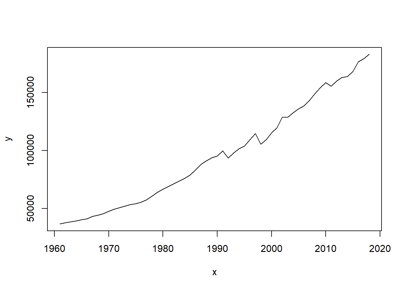
y <- group_by_year$med_stocks
x <- group_by_year$Year
plot(x, y, type = "l")