Join Tables and Analyzing Data

Joining Data

Introduction

I was trying to analyze the snl_actors and snl_casts datasets in order to find out the approximate screen time for male and female SNL actors. We first start by importing the necessary libraries and setting the working directory to point to the location where the spreadsheet is located. Then we read in both the datasets into dataframes. From the snl_casts dataset, we approximate the screen_time for every actor by multiplying the number of episodes the actor appreared in with the season_fraction.

library(tidyverse)
library(ggplot2)
knitr::opts_chunk$set(echo = TRUE, warning=FALSE, message=FALSE)
setwd("D:/MyDocs/Class Slides/DACSS601/601_Spring_2023/posts/_data")
actors <- read.csv("snl_actors.csv")
casts <- read.csv("snl_casts.csv") %>%
  select(-"first_epid", -"last_epid") %>%
  mutate(screen_time = n_episodes * season_fraction)

Join Data

Our actors dataframe has information about actor gender. We create join_one by combining both actors and casts dataframes with an inner join grouping by actor id - aid and summarizing to get total screen time per actor in terms of episodes. We know that actors has a separate row of information for every cast member and guest on snl, while casts contains rows of information for actors only. Performing inner join based on aid will match rows based on aid which guests do not have. Therefore, to perform a sanity check of our join results, we can print number of rows in casts and number of rows in join_one and they must be the same. Afterwards, we get join_two which contains a separate row for every different actor in join_one. Here, we are getting a separate row for every aid by summing the screen times for actors. Thus we can perform a sanity check once again by making sure the length of join_two is the same as the number of unique actors ids in join_one.

join_one <- casts %>% 
  inner_join(actors, by = "aid") %>%
  select(-"update_anchor", -"n_episodes", -"url", -"season_fraction", -"featured", -"type")
head(casts)

               aid sid featured update_anchor n_episodes season_fraction
1 A. Whitney Brown  11     True         False          8       0.4444444
2 A. Whitney Brown  12     True         False         20       1.0000000
3 A. Whitney Brown  13     True         False         13       1.0000000
4 A. Whitney Brown  14     True         False         20       1.0000000
5 A. Whitney Brown  15     True         False         20       1.0000000
6 A. Whitney Brown  16     True         False         20       1.0000000
  screen_time
1    3.555556
2   20.000000
3   13.000000
4   20.000000
5   20.000000
6   20.000000

head(join_one)

               aid sid screen_time gender
1 A. Whitney Brown  11    3.555556   male
2 A. Whitney Brown  12   20.000000   male
3 A. Whitney Brown  13   13.000000   male
4 A. Whitney Brown  14   20.000000   male
5 A. Whitney Brown  15   20.000000   male
6 A. Whitney Brown  16   20.000000   male

print(nrow(casts))

[1] 614

print(nrow(join_one))

[1] 614

join_two <- join_one %>% group_by(aid, gender) %>%
  summarise(total_screen_time = sum(screen_time))
head(join_two)

# A tibble: 6 × 3
# Groups:   aid [6]
  aid              gender total_screen_time
  <chr>            <chr>              <dbl>
1 A. Whitney Brown male               96.6 
2 Abby Elliott     female             76.2 
3 Adam Sandler     male               84.0 
4 Aidy Bryant      female            182   
5 Al Franken       male              192.  
6 Alan Zweibel     male                1.25

print(length(unique(join_one$aid)))

[1] 156

print(nrow(join_two))

[1] 156

Visualization and Analysis

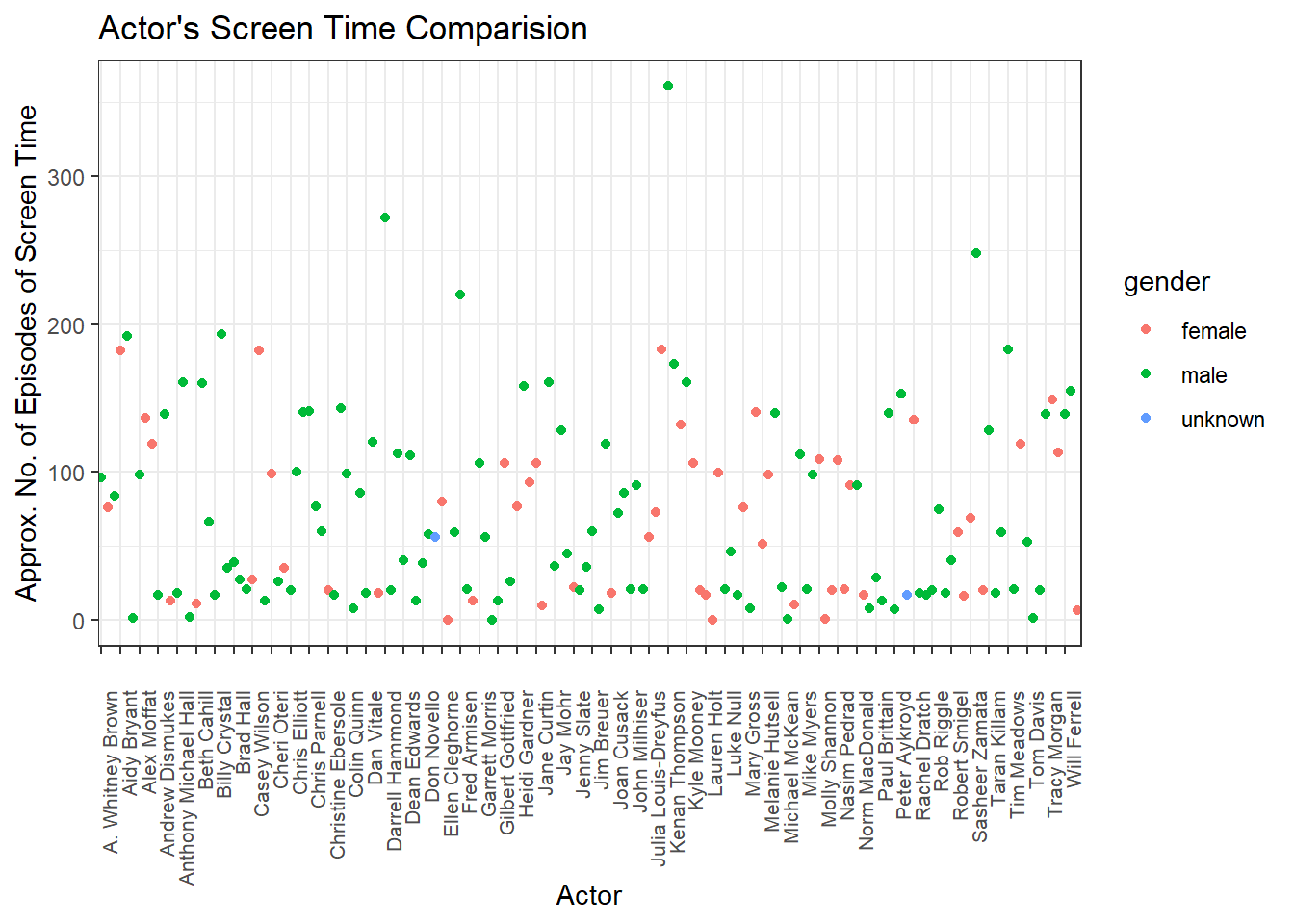
We can visualize the resulting dataframe comparing actor’s screen time and coloring them based on gender to give a good picture of average screen time for male and female snl stars.

join_two %>% 
    ggplot(aes(y=total_screen_time, x=aid, color=gender)) +
    geom_point() +
    theme_bw() +
    theme(axis.text.x = element_text(angle = 90, hjust = 1, margin = margin(t = 0.5, unit = "cm"), size = 8)) +
    scale_x_discrete(breaks = join_two$aid[seq(1, length(join_two$aid), by = 3)]) +
    labs(title = "Actor's Screen Time Comparision", x = "Actor", y = "Approx. No. of Episodes of Screen Time")