Challenge 8 Instructions

challenge_8

railroads

snl

faostat

debt

Joining Data

Author

Sai Pranav Kurly

Published

May 15, 2023

library(tidyverse)
library(ggplot2)

knitr::opts_chunk$set(echo = TRUE, warning=FALSE, message=FALSE)

Challenge Overview

Today’s challenge is to:

read in multiple data sets, and describe the data set using both words and any supporting information (e.g., tables, etc)
tidy data (as needed, including sanity checks)
mutate variables as needed (including sanity checks)
join two or more data sets and analyze some aspect of the joined data

(be sure to only include the category tags for the data you use!)

Read in data

Read in one (or more) of the following datasets, using the correct R package and command.

military marriages ⭐⭐
faostat ⭐⭐
railroads ⭐⭐⭐
fed_rate ⭐⭐⭐
debt ⭐⭐⭐
us_hh ⭐⭐⭐⭐
snl ⭐⭐⭐⭐⭐

I’m planning to use the SNL data:

snl_actors <- read_csv("_data/snl_actors.csv")
head(snl_actors)

# A tibble: 6 × 4
  aid            url           type  gender 
  <chr>          <chr>         <chr> <chr>  
1 Kate McKinnon  /Cast/?KaMc   cast  female 
2 Alex Moffat    /Cast/?AlMo   cast  male   
3 Ego Nwodim     /Cast/?EgNw   cast  unknown
4 Chris Redd     /Cast/?ChRe   cast  male   
5 Kenan Thompson /Cast/?KeTh   cast  male   
6 Carey Mulligan /Guests/?3677 guest andy

dim(snl_actors)

[1] 2306    4

snl_casts <- read_csv("_data/snl_casts.csv")
head(snl_casts)

# A tibble: 6 × 8
  aid                sid featured first_epid last_epid update_…¹ n_epi…² seaso…³
  <chr>            <dbl> <lgl>         <dbl>     <dbl> <lgl>       <dbl>   <dbl>
1 A. Whitney Brown    11 TRUE       19860222        NA FALSE           8   0.444
2 A. Whitney Brown    12 TRUE             NA        NA FALSE          20   1    
3 A. Whitney Brown    13 TRUE             NA        NA FALSE          13   1    
4 A. Whitney Brown    14 TRUE             NA        NA FALSE          20   1    
5 A. Whitney Brown    15 TRUE             NA        NA FALSE          20   1    
6 A. Whitney Brown    16 TRUE             NA        NA FALSE          20   1    
# … with abbreviated variable names ¹update_anchor, ²n_episodes,
#   ³season_fraction

dim(snl_casts)

[1] 614   8

snl_seasons <- read_csv("_data/snl_seasons.csv")
head(snl_seasons)

# A tibble: 6 × 5
    sid  year first_epid last_epid n_episodes
  <dbl> <dbl>      <dbl>     <dbl>      <dbl>
1     1  1975   19751011  19760731         24
2     2  1976   19760918  19770521         22
3     3  1977   19770924  19780520         20
4     4  1978   19781007  19790526         20
5     5  1979   19791013  19800524         20
6     6  1980   19801115  19810411         13

dim(snl_seasons)

[1] 46  5

Briefly describe the data

This dataset contains information on the casts of Saturday Night Live from 1975 to 2020. Each row of this newly created dataframe represents a distinct actor-season pairing, complete with information on the actor and the SNL seasons in which they have appeared. Each row includes information about the actor’s gender, whether they appeared in a specific season, the date of their first episode, the date of their last episode, the number of episodes they’ve appeared in, the percentage of each season they’ve appeared in, a URL for that actor, whether they were a member of the cast or a guest on the show, and whether they were an anchor on weekend update.

Tidy Data (as needed)

We can check for N/A and get rid of them in all the datasets.

snl_actors <- snl_actors %>%
  drop_na()
snl_actors

# A tibble: 2,249 × 4
   aid            url           type  gender 
   <chr>          <chr>         <chr> <chr>  
 1 Kate McKinnon  /Cast/?KaMc   cast  female 
 2 Alex Moffat    /Cast/?AlMo   cast  male   
 3 Ego Nwodim     /Cast/?EgNw   cast  unknown
 4 Chris Redd     /Cast/?ChRe   cast  male   
 5 Kenan Thompson /Cast/?KeTh   cast  male   
 6 Carey Mulligan /Guests/?3677 guest andy   
 7 Marcus Mumford /Guests/?3679 guest male   
 8 Aidy Bryant    /Cast/?AiBr   cast  female 
 9 Steve Higgins  /Crew/?StHi   crew  male   
10 Mikey Day      /Cast/?MiDa   cast  male   
# … with 2,239 more rows

snl_casts <- snl_casts %>%
  select(aid, sid, featured, update_anchor, n_episodes, season_fraction)
snl_casts <- snl_casts %>%
  drop_na()
snl_casts

# A tibble: 614 × 6
   aid                sid featured update_anchor n_episodes season_fraction
   <chr>            <dbl> <lgl>    <lgl>              <dbl>           <dbl>
 1 A. Whitney Brown    11 TRUE     FALSE                  8           0.444
 2 A. Whitney Brown    12 TRUE     FALSE                 20           1    
 3 A. Whitney Brown    13 TRUE     FALSE                 13           1    
 4 A. Whitney Brown    14 TRUE     FALSE                 20           1    
 5 A. Whitney Brown    15 TRUE     FALSE                 20           1    
 6 A. Whitney Brown    16 TRUE     FALSE                 20           1    
 7 Alan Zweibel         5 TRUE     FALSE                  5           0.25 
 8 Sasheer Zamata      39 TRUE     FALSE                 11           0.524
 9 Sasheer Zamata      40 TRUE     FALSE                 21           1    
10 Sasheer Zamata      41 FALSE    FALSE                 21           1    
# … with 604 more rows

snl_seasons <- snl_seasons %>% 
  drop_na()
snl_seasons

# A tibble: 46 × 5
     sid  year first_epid last_epid n_episodes
   <dbl> <dbl>      <dbl>     <dbl>      <dbl>
 1     1  1975   19751011  19760731         24
 2     2  1976   19760918  19770521         22
 3     3  1977   19770924  19780520         20
 4     4  1978   19781007  19790526         20
 5     5  1979   19791013  19800524         20
 6     6  1980   19801115  19810411         13
 7     7  1981   19811003  19820522         20
 8     8  1982   19820925  19830514         20
 9     9  1983   19831008  19840512         19
10    10  1984   19841006  19850413         17
# … with 36 more rows

Join Data

We can join all 3 datasets and then analyze

snl_actors_casts <- snl_actors %>%
  inner_join(snl_casts, by="aid")

snl_actors_casts_seasons <- snl_actors_casts %>%
  inner_join(snl_seasons, by="sid")
snl_actors_casts_seasons

# A tibble: 607 × 13
   aid    url   type  gender   sid featu…¹ updat…² n_epi…³ seaso…⁴  year first…⁵
   <chr>  <chr> <chr> <chr>  <dbl> <lgl>   <lgl>     <dbl>   <dbl> <dbl>   <dbl>
 1 Kate … /Cas… cast  female    37 TRUE    FALSE         5   0.227  2011  2.01e7
 2 Kate … /Cas… cast  female    38 TRUE    FALSE        21   1      2012  2.01e7
 3 Kate … /Cas… cast  female    39 FALSE   FALSE        21   1      2013  2.01e7
 4 Kate … /Cas… cast  female    40 FALSE   FALSE        21   1      2014  2.01e7
 5 Kate … /Cas… cast  female    41 FALSE   FALSE        21   1      2015  2.02e7
 6 Kate … /Cas… cast  female    42 FALSE   FALSE        21   1      2016  2.02e7
 7 Kate … /Cas… cast  female    43 FALSE   FALSE        21   1      2017  2.02e7
 8 Kate … /Cas… cast  female    44 FALSE   FALSE        21   1      2018  2.02e7
 9 Kate … /Cas… cast  female    45 FALSE   FALSE        18   1      2019  2.02e7
10 Kate … /Cas… cast  female    46 FALSE   FALSE        17   1      2020  2.02e7
# … with 597 more rows, 2 more variables: last_epid <dbl>, n_episodes.y <dbl>,
#   and abbreviated variable names ¹featured, ²update_anchor, ³n_episodes.x,
#   ⁴season_fraction, ⁵first_epid

With the below plot we can see how analyze SNL cast by their gender per season

graph <- ggplot(snl_actors_casts_seasons, aes(sid, fill = gender)) +
  geom_bar() +
  labs(
    title = "SNL Cast by Gender per Season",
    x = "Season",
    y = "Count",
    fill = "Gender"
  ) 
graph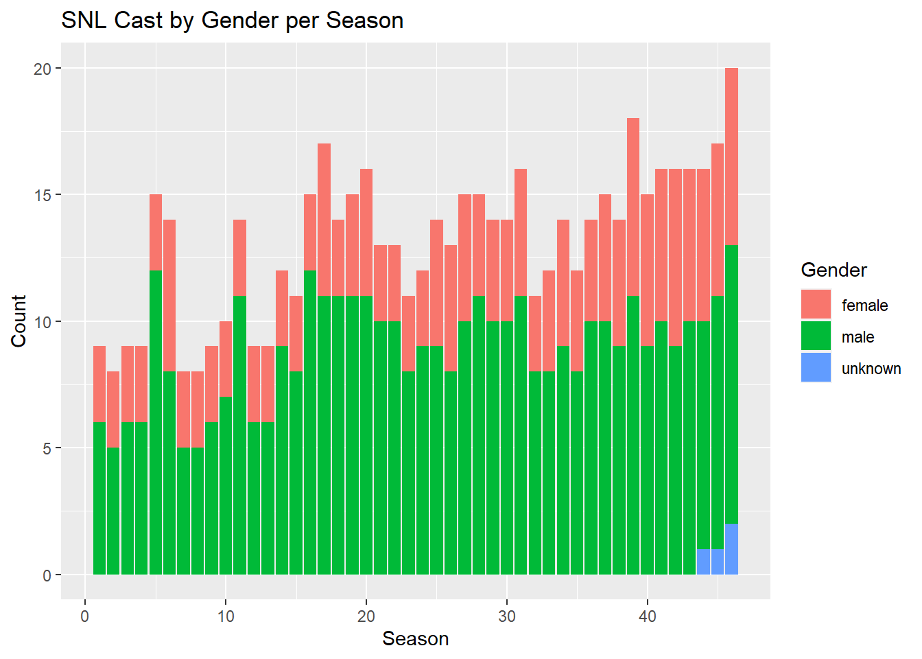

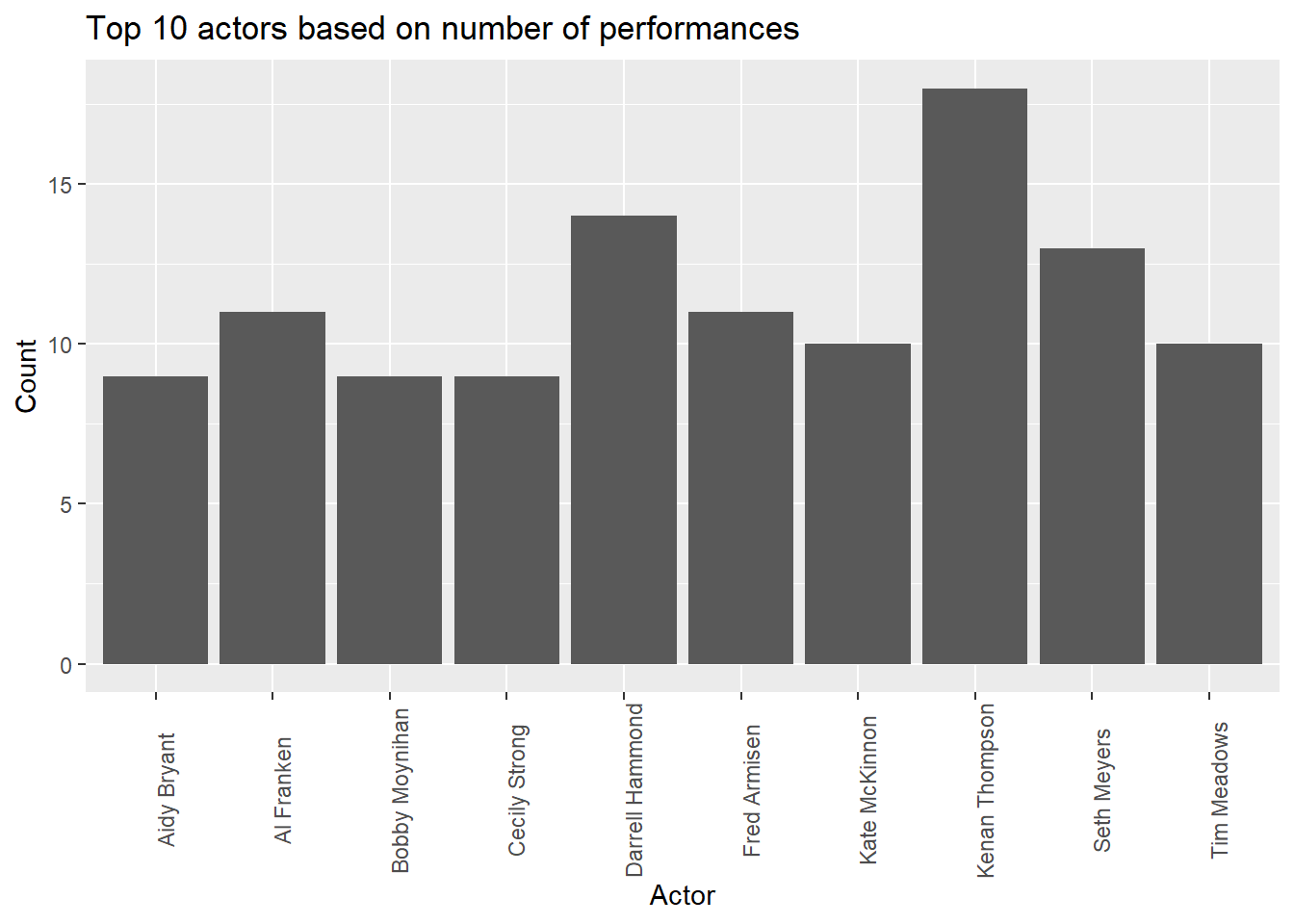
With the below plot we can see the top 10 actors based on number of performances

# Calculate the number of times each actor acted in each year
actor_counts <- snl_actors_casts_seasons %>%
  group_by(aid) %>%
  summarise(count = n())

top_10_actors <- actor_counts %>%
  arrange(desc(count)) %>%
  head(10)

# Create the graph
graph <- ggplot(top_10_actors, aes(x = aid, y = count)) +
  geom_bar(stat = "identity") +
  labs(
    title = "Top 10 actors based on number of performances",
    x = "Actor",
    y = "Count",
  ) + theme(axis.text.x = element_text(angle = 90))
graph