library(ggplot2)
library(dplyr)
library(lubridate)
library(leaflet)
library(tidyverse)
knitr::opts_chunk$set(echo = TRUE, warning=FALSE, message=FALSE)Final Project Assignment#2: Sai Pranav Kurly
final_Project_assignment_2
final_project_data_description
Exploratory Analysis and Visualization
Part 1. Introduction
- Dataset(s) Introduction:
The Boston Crime Dataset, also known as the Boston Crime Incident Reports, is a dataset that contains information about reported incidents of crime in the city of Boston, Massachusetts, USA. It provides a detailed record of criminal activities and incidents that have occurred within the city. The dataset includes various attributes related to each reported crime, such as the type of offense, location, date and time of occurrence, and other relevant details. The information is collected and maintained by the Boston Police Department, which aims to promote transparency and public awareness regarding crime trends and patterns in the city. Researchers, analysts, and data enthusiasts often utilize the Boston Crime Dataset to study crime patterns, develop predictive models, and gain insights into criminal activities within the city. It can be used for various purposes, such as identifying high-crime areas, evaluating the effectiveness of law enforcement strategies, or understanding the impact of crime on different neighborhoods.
- What questions do you like to answer with this dataset(s)?
Some of the questions that I would like to answer and figure out are:
How have crime rates changed over the years in different districts of Boston? Is there a correlation between certain types of crimes and specific days of the week or months of the year? *Are there any noticeable spatial patterns or hotspots of crime in Boston?
Part 2. Describe the data set(s)
This part contains both a coding and a storytelling component.
In the coding component, you should:
- read the dataset;
I want the latest data which can only be found on the Boston PD website, hence I am combining all the data that I downloaded from the website first.
folder_path <- "SaipranavKurly_FinalProjectData/"
file_list <- list.files(folder_path)
file_list <- sort(file_list)
combined_data <- data.frame()
for (file_name in file_list) {
    if(file_name != 'Offense_Codes.csv' & file_name != 'Combined_Dataset.csv'){
          file_path <- file.path(folder_path, file_name)
    file_data <- read.csv(file_path)
    combined_data <- rbind(combined_data, file_data)
    }
}
combined_file_path <- file.path(folder_path, "Combined_Dataset.csv")
write.csv(combined_data, combined_file_path, row.names = FALSE)
- (optional) If you have multiple dataset(s) you want to work with, you should combine these datasets at this step.
- (optional) If your dataset is too big (for example, it contains too many variables/columns that may not be useful for your analysis), you may want to subset the data just to include the necessary variables/columns.Reading the dataset and merging:
crime_dataset <- read.csv("SaipranavKurly_FinalProjectData/Combined_Dataset.csv")
offence_codes_dataset <- read.csv("SaipranavKurly_FinalProjectData/Offense_Codes.csv")
names(offence_codes_dataset) <- c("OFFENSE_CODE", "OFFENCE_NAME")
crime_dataset <- merge(crime_dataset, offence_codes_dataset, by = "OFFENSE_CODE", all.x = TRUE)
present the descriptive information of the dataset(s) using the functions in Challenges 1, 2, and 3;
- for examples: dim(), length(unique()), head();
dim(crime_dataset)[1] 531744 18length(unique(crime_dataset))[1] 18head(crime_dataset)conduct summary statistics of the dataset(s); especially show the basic statistics (min, max, mean, median, etc.) for the variables you are interested in.
summary(crime_dataset) OFFENSE_CODE INCIDENT_NUMBER OFFENSE_CODE_GROUP OFFENSE_DESCRIPTION
Min. : 100 Length:531744 Mode:logical Length:531744
1st Qu.: 801 Class :character NA's:531744 Class :character
Median : 3005 Mode :character Mode :character
Mean : 2259
3rd Qu.: 3115
Max. :99999
DISTRICT REPORTING_AREA SHOOTING OCCURRED_ON_DATE
Length:531744 Min. : 0.0 Min. :0.00000 Length:531744
Class :character 1st Qu.:170.0 1st Qu.:0.00000 Class :character
Mode :character Median :350.0 Median :0.00000 Mode :character
Mean :378.8 Mean :0.01334
3rd Qu.:531.0 3rd Qu.:0.00000
Max. :962.0 Max. :1.00000
NA's :130755
YEAR MONTH DAY_OF_WEEK HOUR
Min. :2019 Min. : 1.000 Length:531744 Min. : 0.00
1st Qu.:2019 1st Qu.: 4.000 Class :character 1st Qu.: 9.00
Median :2020 Median : 7.000 Mode :character Median :14.00
Mean :2020 Mean : 6.568 Mean :12.82
3rd Qu.:2021 3rd Qu.: 9.000 3rd Qu.:18.00
Max. :2022 Max. :12.000 Max. :23.00
UCR_PART STREET Lat Long
Mode:logical Length:531744 Min. : 0.00 Min. :-71.35
NA's:531744 Class :character 1st Qu.:42.30 1st Qu.:-71.10
Mode :character Median :42.33 Median :-71.08
Mean :42.32 Mean :-71.08
3rd Qu.:42.35 3rd Qu.:-71.06
Max. :42.46 Max. : 0.00
NA's :20640 NA's :20640
Location OFFENCE_NAME
Length:531744 Length:531744
Class :character Class :character
Mode :character Mode :character
Storytelling:
The Dataset contains the following columns and below are the descriptions:
- Incident Number: Internal report number for each incident, non-null value.
- Offense Code: Numerical code representing the offense description.
- Offense Code Group: High-level group name for the offense code.
- Offense Description: Detailed description and internal categorization of the offense.
- District: District where the crime occurred.
- Reporting Area: Number of the reporting area where the crime occurred.
- Shooting: Numerical value indicating if a shooting took place.
- Occurred on Date: Date and time of when the crime occurred.
- Year: Year when the crime occurred.
- Month: Month when the crime occurred.
- Day of Week: Day of the week when the crime occurred.
- Hour: Hour when the crime occurred.
- UCR Part: Universal Crime Reporting Part Number.
- Street: Street name where the crime occurred.
- Lat: Latitude coordinate of the crime location.
- Long: Longitude coordinate of the crime location.
- Location - Gives the location of where the crime has taken place.
It consists of crimes from 2019 to 2023 and has about 2738464 crimes in total.
3. Plan for Visualization
- Briefly describe what data analyses (please the special note on statistics in the next section) and visualizations you plan to conduct to answer the research questions you proposed above.
Currently, I am planning to to analyze the following using the dataset:
Crime Distribution and Frequency:
Create a bar chart to depict the distribution of crime types in Boston.
Additionally, I am also going to determine the most and least common crime categories.
Finally, I plan to also visualize which streets have the highest crime.
Temporal Patterns and Trends:
Using line graphs or time series plots, plot the number of reported crimes over time (monthly or yearly).
Identify any notable trends or patterns in crime rates over time. For example, at what hour do mouse crimes happen at.
Seasonal Variation in Crime:
Aggregate the data by month or season to see if there are seasonal variations in crime rates.
To compare the distribution of crimes across seasons, create box plots or violin plots.
Geographic Crime Hotspots:
Identify high-crime areas in Boston using geospatial visualization techniques.
To visualize crime density, plot crime incidents on a map with markers or heatmaps.
- Explain why you choose to conduct these specific data analyses and visualizations. In other words, how do such types of statistics or graphs (see the R Gallery) help you answer specific questions? For example, how can a bivariate visualization reveal the relationship between two variables, or how does a linear graph of variables over time present the pattern of development?
The distribution of crime types can be represented visually using bar charts or pie charts. They give a clear overview of the most common and least common crime categories, making it simple to identify major crime trends. Line graphs and time series plots are useful for examining how crime rates change over time. In crime data, they reveal trends, patterns, and cyclical behavior. These visualizations aid in the identification of long-term trends, seasonal patterns, and unexpected changes in crime rates.Box plots and violin plots allow for the comparison of crime rates across seasons. They provide insights into the distribution of crime incidents during specific periods and aid in determining whether there are significant seasonal differences in crime rates.
- If you plan to conduct specific data analyses and visualizations, describe how do you need to process and prepare the tidy data.
To clean the dataset, I am removing all the rows where the OFFENCE_NAMES are NA. Additionally there are a few categories which I feel are not of much use to analyze the crimes in boston and I have removed them as well. I also plan to mutate and add additional columns like months from the date column during the preprocessing step so that it will make it easier to plot graphs.
Cleaning the dataset:
crime_dataset <- crime_dataset[crime_dataset$OFFENCE_NAME != "INVESTIGATE PERSON", ]
crime_dataset <- crime_dataset[crime_dataset$OFFENCE_NAME != "INVESTIGATE PROPERTY", ]
crime_dataset <- crime_dataset[complete.cases(crime_dataset$OFFENCE_NAME), ]
4. Analyses and Visualizations
Crime Distribution and Frequency
crime_freq <- crime_dataset %>%
  group_by(OFFENCE_NAME) %>%
  summarize(crime_count = n()) %>%
  arrange(desc(crime_count))
crime_freq
Bar chart of top 10 crime types
ggplot(head(crime_freq,10), aes(x = reorder(OFFENCE_NAME, -crime_count), y = crime_count)) +
  geom_bar(stat = "identity", fill = "lightpink") +
  labs(x = "Crime Types", y = "Frequency", title = "Crime Distribution in Boston") +
  theme(axis.text.x = element_text(angle = 45, hjust = 1))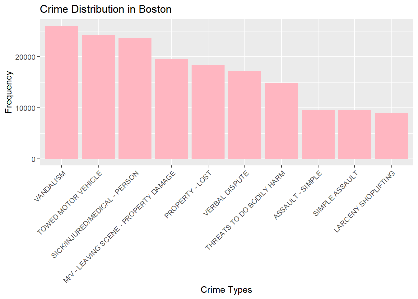
Bar chart of bottom 10 crime types
ggplot(tail(crime_freq,10), aes(x = reorder(OFFENCE_NAME, -crime_count), y = crime_count)) +
  geom_bar(stat = "identity", fill = "lightgreen") +
  labs(x = "Crime Types", y = "Frequency", title = "Crime Distribution in Boston") +
  theme(axis.text.x = element_text(angle = 45, hjust = 1))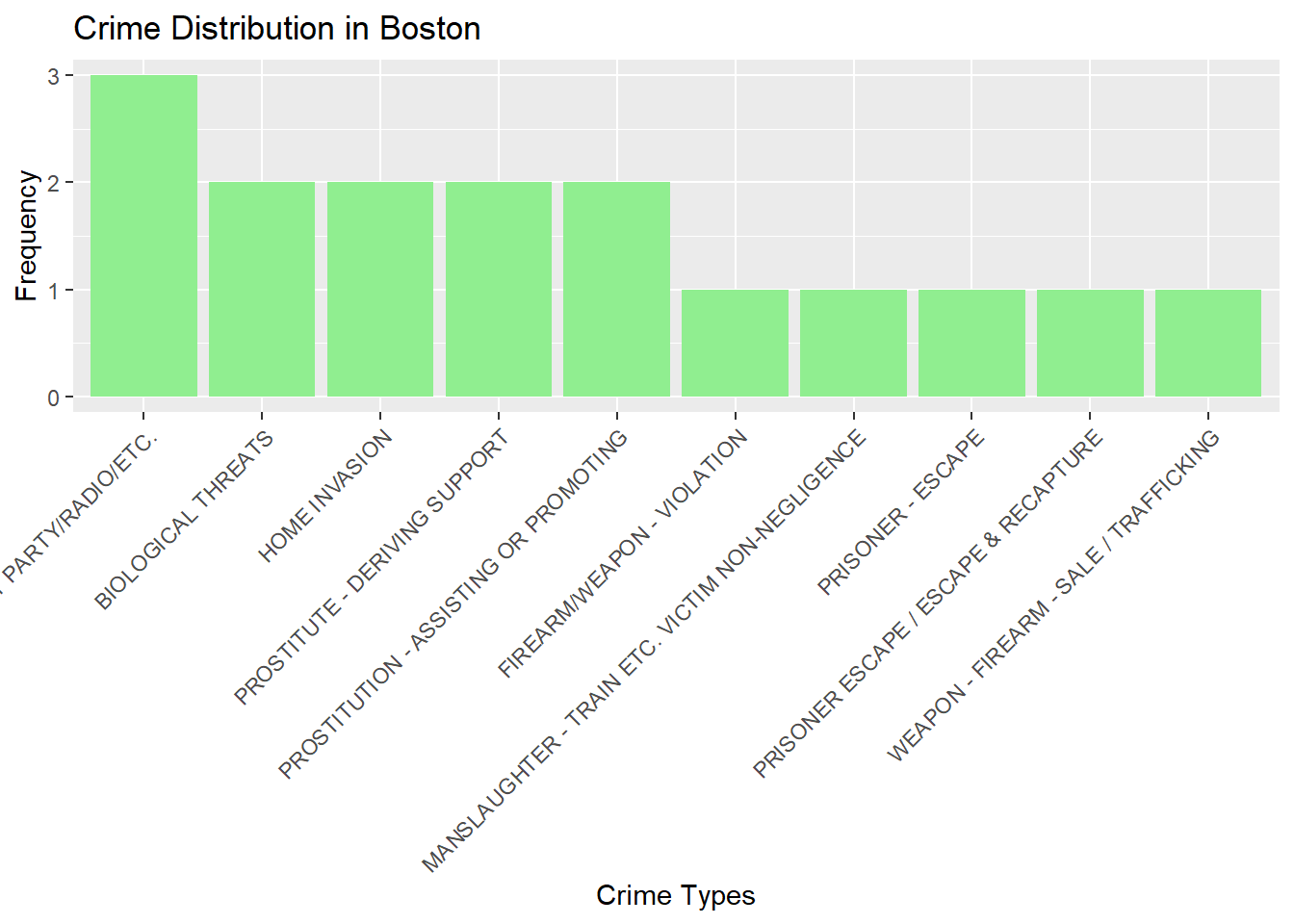
Line plot of crime counts over time:
crime_dates <- crime_dataset %>%
  mutate(Date = as.Date(OCCURRED_ON_DATE)) %>%
  count(Date) %>%
  mutate(Year = year(Date), Month = month(Date, label = TRUE))
ggplot(crime_dates, aes(x = Date, y = n)) +
  geom_line(color = "steelblue") +
labs(x = "Date", y = "Number of Crimes", title = "Temporal Patterns of Reported Crimes") 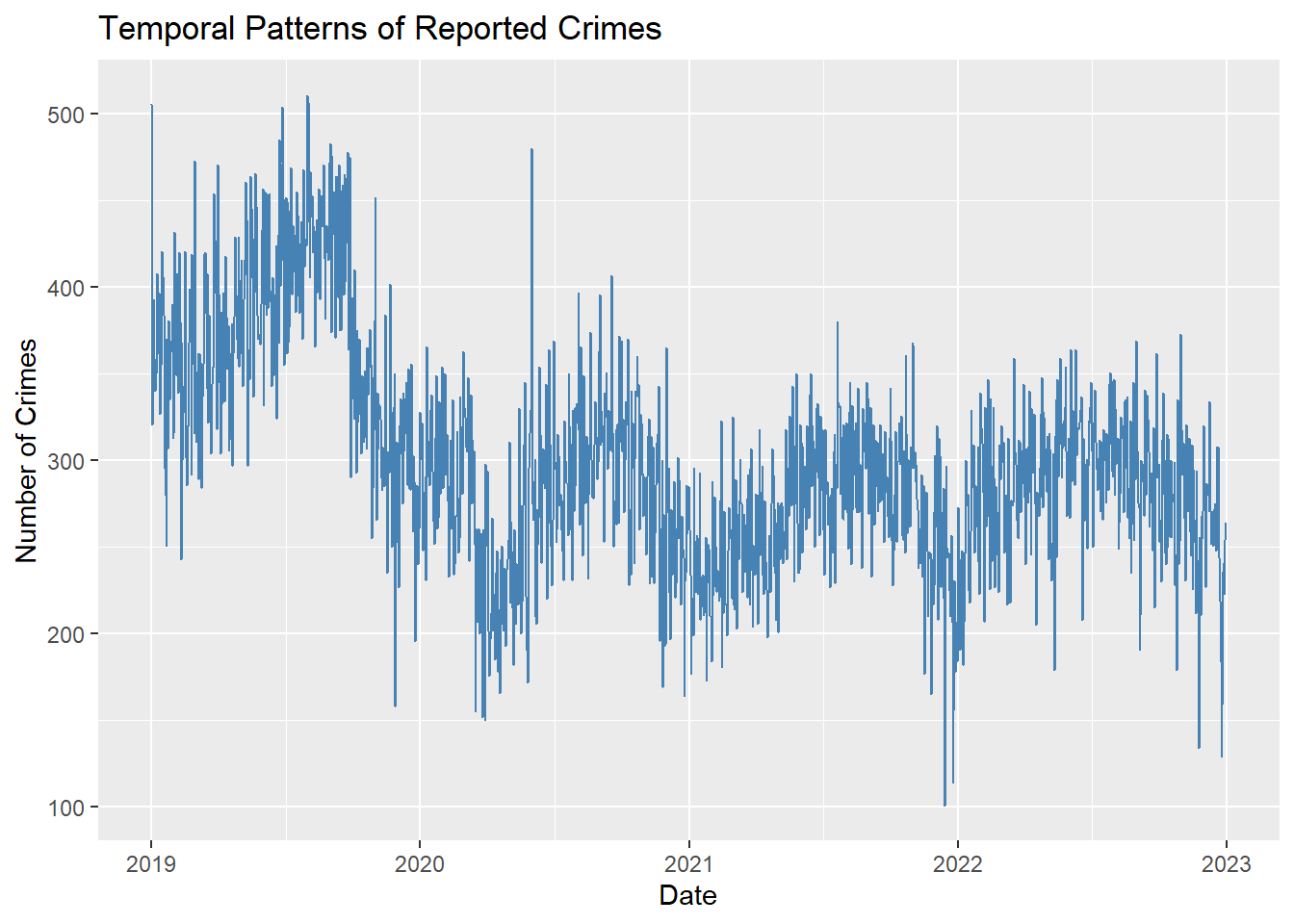
Bar graph of the crimes during different hours of the day:
crime_hour_plot <- ggplot(crime_dataset, aes(x = HOUR)) +
  geom_bar(fill = "lightsalmon", color = "black") +
  labs(x = "HOUR", y = "Number of Crimes", title = "Crimes During Different Hours")
crime_hour_plot +
theme(axis.text.x = element_text(angle = 90, hjust = 1)) 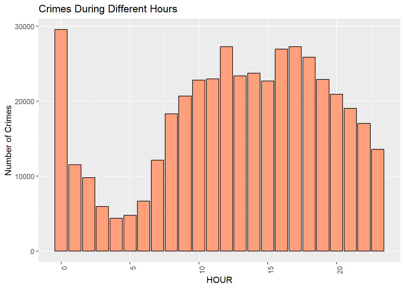
crime_season <- crime_dataset %>%
  mutate(Season = case_when(
    month(OCCURRED_ON_DATE) %in% c(3, 4, 5) ~ "Spring",
    month(OCCURRED_ON_DATE) %in% c(6, 7, 8) ~ "Summer",
    month(OCCURRED_ON_DATE) %in% c(9, 10, 11) ~ "Autumn",
    TRUE ~ "Winter"
  )) %>%
  group_by(Season) %>%
  summarise(Count = n())
Bar plot of crime distribution across seasons:
ggplot(crime_season, aes(x = Season, y = Count)) +
  geom_bar(stat = "identity", fill = "skyblue") +
labs(x = "Season", y = "Number of Crimes", title = "Crime Counts by Season") 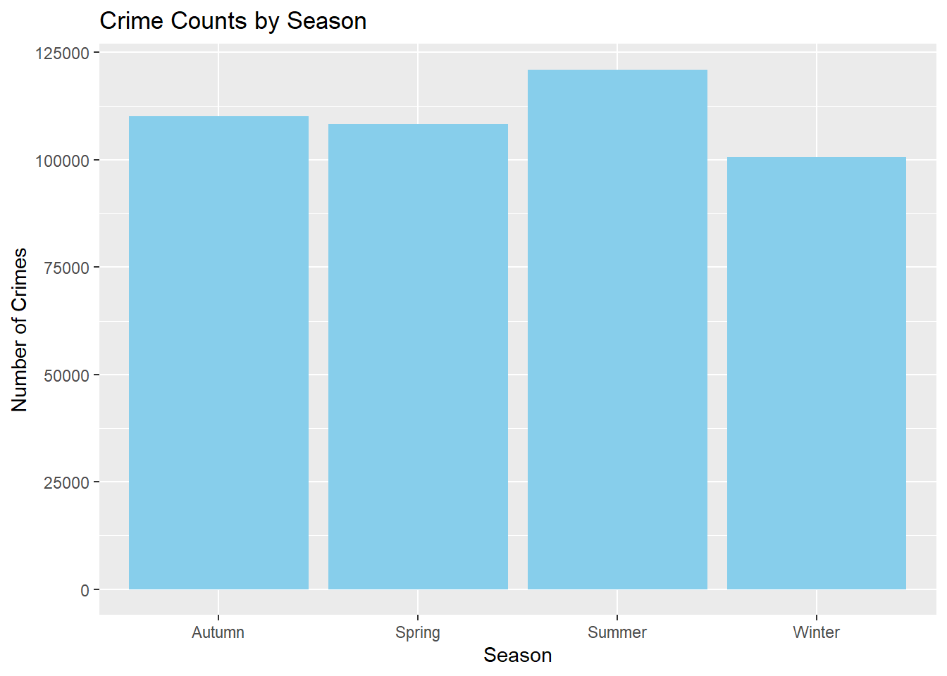
Geographic Crime Hotspots based on Murder,Burglary and Robbery:
crimes_map <- crime_dataset %>%
  filter(str_detect(OFFENCE_NAME, regex("MURDER|BURGLARY|ROBBERY", ignore_case = TRUE)))
basemap <- addTiles(leaflet())
colors = c('Red', 'Green', 'Blue')
i = 1
crimes <- basemap
for (crime in c('MURDER', 'BURGLARY', 'ROBBERY'))
{
  c <- crimes_map[grepl(crime, crimes_map$OFFENCE_NAME, ignore.case = TRUE), ]
  crimes <- addCircleMarkers(setView(crimes, lng = -71.08, lat = 42.33, zoom = 12), lng = c$Long, lat = c$Lat, radius = 1, fillOpacity = 6, color = colors[i])
  i <- i + 1
}
crimes