Exploring the Birds dataset

Reading in data and creating a post

Code

library(tidyverse)

knitr::opts_chunk$set(echo = TRUE, warning=FALSE, message=FALSE)

Challenge Overview

Today’s challenge is to

1. read in a dataset, and

2. describe the dataset using both words and any supporting information (e.g., tables, etc)

Read in the Data

Read in one (or more) of the following data sets, using the correct R package and command.

• railroad_2012_clean_county.csv ⭐
• birds.csv ⭐⭐
• FAOstat*.csv ⭐⭐
• wild_bird_data.xlsx ⭐⭐⭐
• StateCounty2012.xls ⭐⭐⭐⭐

Find the _data folder, located inside the posts folder. Then you can read in the data, using either one of the readr standard tidy read commands, or a specialized package such as readxl.

Code

birds <- read_csv('_data/birds.csv', show_col_types = FALSE)

Code

birds

# A tibble: 30,977 × 14
   Domain Cod…¹ Domain Area …² Area  Eleme…³ Element Item …⁴ Item  Year …⁵  Year
   <chr>        <chr>    <dbl> <chr>   <dbl> <chr>     <dbl> <chr>   <dbl> <dbl>
 1 QA           Live …       2 Afgh…    5112 Stocks     1057 Chic…    1961  1961
 2 QA           Live …       2 Afgh…    5112 Stocks     1057 Chic…    1962  1962
 3 QA           Live …       2 Afgh…    5112 Stocks     1057 Chic…    1963  1963
 4 QA           Live …       2 Afgh…    5112 Stocks     1057 Chic…    1964  1964
 5 QA           Live …       2 Afgh…    5112 Stocks     1057 Chic…    1965  1965
 6 QA           Live …       2 Afgh…    5112 Stocks     1057 Chic…    1966  1966
 7 QA           Live …       2 Afgh…    5112 Stocks     1057 Chic…    1967  1967
 8 QA           Live …       2 Afgh…    5112 Stocks     1057 Chic…    1968  1968
 9 QA           Live …       2 Afgh…    5112 Stocks     1057 Chic…    1969  1969
10 QA           Live …       2 Afgh…    5112 Stocks     1057 Chic…    1970  1970
# … with 30,967 more rows, 4 more variables: Unit <chr>, Value <dbl>,
#   Flag <chr>, `Flag Description` <chr>, and abbreviated variable names
#   ¹​`Domain Code`, ²​`Area Code`, ³​`Element Code`, ⁴​`Item Code`, ⁵​`Year Code`

Add any comments or documentation as needed. More challenging data sets may require additional code chunks and documentation.

Describe the data

Using a combination of words and results of R commands, can you provide a high level description of the data? Describe as efficiently as possible where/how the data was (likely) gathered, indicate the cases and variables (both the interpretation and any details you deem useful to the reader to fully understand your chosen data).

Code

dim(birds)

[1] 30977    14

The data has 30977 rows and 14 columns (variables)

Code

colnames(birds)

 [1] "Domain Code"      "Domain"           "Area Code"        "Area"            
 [5] "Element Code"     "Element"          "Item Code"        "Item"            
 [9] "Year Code"        "Year"             "Unit"             "Value"           
[13] "Flag"             "Flag Description"

The columns (variables) in our data are listed above.

Code

spec(birds)

cols(
  `Domain Code` = col_character(),
  Domain = col_character(),
  `Area Code` = col_double(),
  Area = col_character(),
  `Element Code` = col_double(),
  Element = col_character(),
  `Item Code` = col_double(),
  Item = col_character(),
  `Year Code` = col_double(),
  Year = col_double(),
  Unit = col_character(),
  Value = col_double(),
  Flag = col_character(),
  `Flag Description` = col_character()
)

This helps us understand the datatype of the variables we have.

Code

birds%>%select(Item)%>%n_distinct()

[1] 5

Code

birds%>%select(Item)%>%unique()

# A tibble: 5 × 1
  Item                  
  <chr>                 
1 Chickens              
2 Ducks                 
3 Geese and guinea fowls
4 Turkeys               
5 Pigeons, other birds  

The dataset contains 5 unique values in the variable ‘Items’. These seem to poultry birds from a first glance.

Code

birds%>%select(Area)%>%n_distinct()

[1] 248

Code

birds%>%select(Area)%>%unique()

# A tibble: 248 × 1
   Area               
   <chr>              
 1 Afghanistan        
 2 Albania            
 3 Algeria            
 4 American Samoa     
 5 Angola             
 6 Antigua and Barbuda
 7 Argentina          
 8 Armenia            
 9 Aruba              
10 Australia          
# … with 238 more rows

The dataset contains 248 unique values in the variable ‘Area’ i.e. it contains data from across 248 countries

Code

library(ggplot2)
ggplot(data = birds, aes(x = Item)) + 
  geom_bar()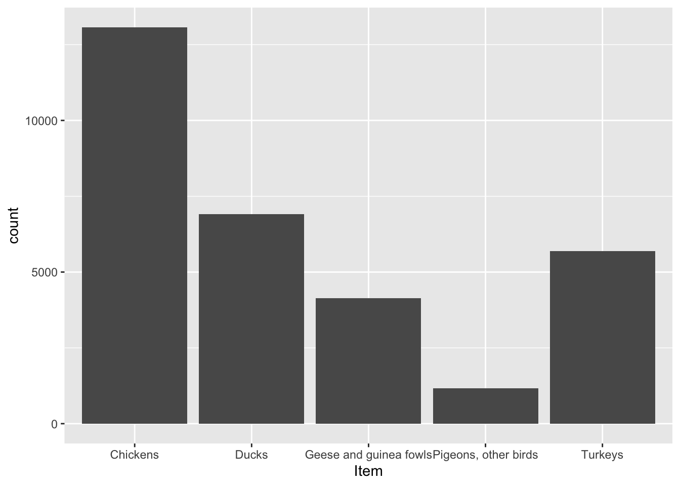

This graph helps us understand the distribution of birds in our dataset. As we can see, chicken is the most popular bird in our dataset.