Challenge 2 : Wrangling and exploring the bird dataset

We dive deeper into the birds dataset and use methods like summarise(), filter() and groupby() to wrangle data

Code

library(tidyverse)

knitr::opts_chunk$set(echo = TRUE, warning=FALSE, message=FALSE)

Challenge Overview

Today’s challenge is to

1. read in a data set, and describe the data using both words and any supporting information (e.g., tables, etc)
2. provide summary statistics for different interesting groups within the data, and interpret those statistics

For this challenge I read in the birds dataset which contains information about poultry domesticated in various regions.

Read in the Data

Code

bird_dataset<-read_csv("_data/birds.csv", show_col_types = FALSE)
bird_dataset

We clean all variables with the word “code” in the name as these variables are only unique identifiers for other variables.

Code

bird_dataset_cleaned<-bird_dataset%>%select(-c(contains("Code")))
bird_dataset_cleaned

Describe the data

We now try to describe the data and further filter the data if the necessary.

We first find the number of unique values in each variable

Code

length(unique(bird_dataset_cleaned$Domain))

[1] 1

Code

length(unique(bird_dataset_cleaned$Area))

[1] 248

Code

length(unique(bird_dataset_cleaned$Element))

[1] 1

Code

length(unique(bird_dataset_cleaned$Item))

[1] 5

Code

length(unique(bird_dataset_cleaned$Year))

[1] 58

Code

length(unique(bird_dataset_cleaned$Unit))

[1] 1

Code

length(unique(bird_dataset_cleaned$Value))

[1] 11496

Code

length(unique(bird_dataset_cleaned$Flag))

[1] 6

Code

length(unique(bird_dataset_cleaned$`Flag Description`))

[1] 6

As we can see that Domain, Element and Unit have only 1 unique value, they can also be dropped

Code

bird_dataset_cleaned<-bird_dataset_cleaned%>%select(-c(Domain, Element, Unit))

Next let us try to find the unique poultry sold.

Code

unique(bird_dataset_cleaned$Item)

[1] "Chickens"               "Ducks"                  "Geese and guinea fowls"
[4] "Turkeys"                "Pigeons, other birds"  

We have 5 categories of poultries

Grouped Summary Statistics

Distribution of stocks, grouped by Poultry Type

Lets first try to see the distribution of the 5 types of poultry by calculating the sum of each of them.

Code

bird_dataset_cleaned%>%
  group_by(Item)%>%
  summarise(total_stocks = sum(Value, na.rm = TRUE),
            avg_stocks = mean(Value, na.rm = TRUE),
            median_stocks = median(Value, na.rm = TRUE),
            std_deviation = sd(Value, na.rm = TRUE),
            min_stock = min(Value, na.rm = TRUE),
            max_stock = max(Value, na.rm = TRUE),)

We can see that Chickens is the most domesticated form of poultry at a total value of 2696862583. The average stock of chicken is 207930.808 across Areas and Years. Similar information can be seen for the other types of poultry

Distribution of stocks, grouped by Decade

Let us try to group the data set by decade and try to find information about it.

Code

bird_dataset_cleaned['decade_code'] <- floor((bird_dataset_cleaned$Year)/10)*10
bird_dataset_cleaned

Code

bird_grpd_decade<-bird_dataset_cleaned%>%
  group_by(decade_code)%>%
  summarise(total_stocks = sum(Value, na.rm = TRUE),
            avg_stocks = mean(Value, na.rm = TRUE),
            median_stocks = median(Value, na.rm = TRUE),
            std_deviation = sd(Value, na.rm = TRUE),
            min_stock = min(Value, na.rm = TRUE),
            max_stock = max(Value, na.rm = TRUE),)

bird_grpd_decade

Code

plot(bird_grpd_decade$total_stocks, bird_grpd_decade$decade_code, type = "b", xlab = "Total Poultry stocks", ylab = "Decade")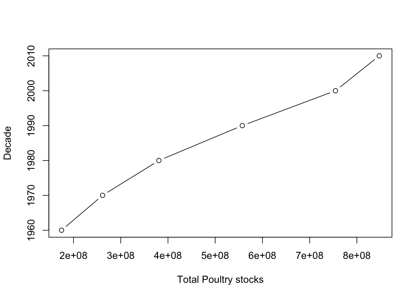

We can see that the total poultry stock has increased almost linearly over the decades, with the highest being in 2010s and the lowest being in the 1960s

Distribution of stocks, grouped by Area and Poultry Type

Next lets try to find the distribution of the different types of poultry across different regions

Code

bird_grp_itm_area<-bird_dataset_cleaned%>%
  group_by(Area, Item)%>%
  summarise(total_stocks = sum(Value, na.rm = TRUE), 
            avg_stocks = mean(Value, na.rm = TRUE),
            median_stocks = median(Value, na.rm = TRUE),
            std_deviation = sd(Value, na.rm = TRUE),
            min_stock = min(Value, na.rm = TRUE),
            max_stock = max(Value, na.rm = TRUE),)

bird_grp_itm_area

We can see all the statistics in the table above. For example Afghanistan has had a total of 469727 chickens.

Distribution of chicken stocks, grouped by Decade

Since Chickens are he most popular of the 5 poultry types, lets explore chicken further. We now filter the data by chicken

Code

chicken_dataset<-filter(bird_dataset_cleaned, Item == "Chickens")%>%select(-c(Item))
chicken_dataset

Code

chicken_dataset_grpd_area<-chicken_dataset%>%
  group_by(decade_code)%>%
  summarise(total_stocks = sum(Value, na.rm = TRUE), 
            avg_stocks = mean(Value, na.rm = TRUE),
            median_stocks = median(Value, na.rm = TRUE),
            std_deviation = sd(Value, na.rm = TRUE),
            min_stock = min(Value, na.rm = TRUE),
            max_stock = max(Value, na.rm = TRUE),)

chicken_dataset_grpd_area

Code

plot(chicken_dataset_grpd_area$total_stocks, chicken_dataset_grpd_area$decade_code, type = "b", xlab = "Total Chicken stocks", ylab = "Decade")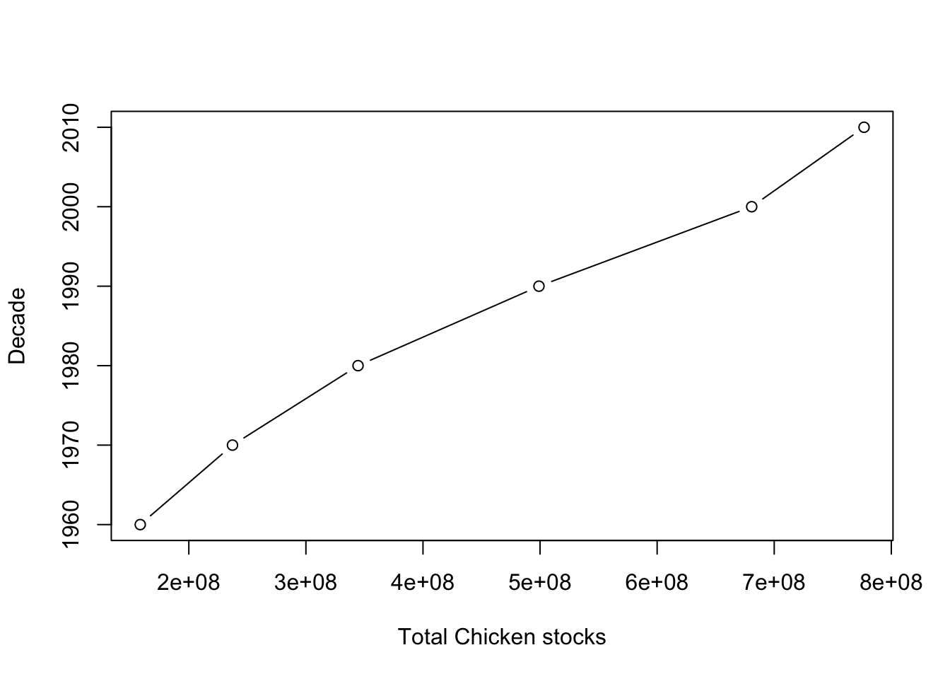

We can see that the total chicken stock has also increased almost linearly over the decades, with the highest being in 2010s and the lowest being in the 1960s