library(tidyverse)
library(ggplot2)
knitr::opts_chunk$set(echo = TRUE, warning=FALSE, message=FALSE)Visualizing Time and Relationships for Hotel Booking Data
Challenge Overview
Today’s challenge is to:
- read in a data set, and describe the data set using both words and any supporting information (e.g., tables, etc)
- tidy data (as needed, including sanity checks)
- mutate variables as needed (including sanity checks)
- create at least one graph including time (evolution)
- try to make them “publication” ready (optional)
- Explain why you choose the specific graph type
- Create at least one graph depicting part-whole or flow relationships
- try to make them “publication” ready (optional)
- Explain why you choose the specific graph type
R Graph Gallery is a good starting point for thinking about what information is conveyed in standard graph types, and includes example R code.
(be sure to only include the category tags for the data you use!)
Read in data
Read in one (or more) of the following datasets, using the correct R package and command.
- debt ⭐
- fed_rate ⭐⭐
- abc_poll ⭐⭐⭐
- usa_hh ⭐⭐⭐
- hotel_bookings ⭐⭐⭐⭐
- AB_NYC ⭐⭐⭐⭐⭐
hotel_data <- read.csv("_data/hotel_bookings.csv")
hotel_dataBriefly describe the data
hotel_data %>% colnames() [1] "hotel" "is_canceled"
[3] "lead_time" "arrival_date_year"
[5] "arrival_date_month" "arrival_date_week_number"
[7] "arrival_date_day_of_month" "stays_in_weekend_nights"
[9] "stays_in_week_nights" "adults"
[11] "children" "babies"
[13] "meal" "country"
[15] "market_segment" "distribution_channel"
[17] "is_repeated_guest" "previous_cancellations"
[19] "previous_bookings_not_canceled" "reserved_room_type"
[21] "assigned_room_type" "booking_changes"
[23] "deposit_type" "agent"
[25] "company" "days_in_waiting_list"
[27] "customer_type" "adr"
[29] "required_car_parking_spaces" "total_of_special_requests"
[31] "reservation_status" "reservation_status_date" We see that there are 32 variables in the dataset. Lets have a look at the summary for each variable of the dataset below.
hotel_data %>% summary() hotel is_canceled lead_time arrival_date_year
Length:119390 Min. :0.0000 Min. : 0 Min. :2015
Class :character 1st Qu.:0.0000 1st Qu.: 18 1st Qu.:2016
Mode :character Median :0.0000 Median : 69 Median :2016
Mean :0.3704 Mean :104 Mean :2016
3rd Qu.:1.0000 3rd Qu.:160 3rd Qu.:2017
Max. :1.0000 Max. :737 Max. :2017
arrival_date_month arrival_date_week_number arrival_date_day_of_month
Length:119390 Min. : 1.00 Min. : 1.0
Class :character 1st Qu.:16.00 1st Qu.: 8.0
Mode :character Median :28.00 Median :16.0
Mean :27.17 Mean :15.8
3rd Qu.:38.00 3rd Qu.:23.0
Max. :53.00 Max. :31.0
stays_in_weekend_nights stays_in_week_nights adults
Min. : 0.0000 Min. : 0.0 Min. : 0.000
1st Qu.: 0.0000 1st Qu.: 1.0 1st Qu.: 2.000
Median : 1.0000 Median : 2.0 Median : 2.000
Mean : 0.9276 Mean : 2.5 Mean : 1.856
3rd Qu.: 2.0000 3rd Qu.: 3.0 3rd Qu.: 2.000
Max. :19.0000 Max. :50.0 Max. :55.000
children babies meal country
Min. : 0.0000 Min. : 0.000000 Length:119390 Length:119390
1st Qu.: 0.0000 1st Qu.: 0.000000 Class :character Class :character
Median : 0.0000 Median : 0.000000 Mode :character Mode :character
Mean : 0.1039 Mean : 0.007949
3rd Qu.: 0.0000 3rd Qu.: 0.000000
Max. :10.0000 Max. :10.000000
NA's :4
market_segment distribution_channel is_repeated_guest
Length:119390 Length:119390 Min. :0.00000
Class :character Class :character 1st Qu.:0.00000
Mode :character Mode :character Median :0.00000
Mean :0.03191
3rd Qu.:0.00000
Max. :1.00000
previous_cancellations previous_bookings_not_canceled reserved_room_type
Min. : 0.00000 Min. : 0.0000 Length:119390
1st Qu.: 0.00000 1st Qu.: 0.0000 Class :character
Median : 0.00000 Median : 0.0000 Mode :character
Mean : 0.08712 Mean : 0.1371
3rd Qu.: 0.00000 3rd Qu.: 0.0000
Max. :26.00000 Max. :72.0000
assigned_room_type booking_changes deposit_type agent
Length:119390 Min. : 0.0000 Length:119390 Length:119390
Class :character 1st Qu.: 0.0000 Class :character Class :character
Mode :character Median : 0.0000 Mode :character Mode :character
Mean : 0.2211
3rd Qu.: 0.0000
Max. :21.0000
company days_in_waiting_list customer_type adr
Length:119390 Min. : 0.000 Length:119390 Min. : -6.38
Class :character 1st Qu.: 0.000 Class :character 1st Qu.: 69.29
Mode :character Median : 0.000 Mode :character Median : 94.58
Mean : 2.321 Mean : 101.83
3rd Qu.: 0.000 3rd Qu.: 126.00
Max. :391.000 Max. :5400.00
required_car_parking_spaces total_of_special_requests reservation_status
Min. :0.00000 Min. :0.0000 Length:119390
1st Qu.:0.00000 1st Qu.:0.0000 Class :character
Median :0.00000 Median :0.0000 Mode :character
Mean :0.06252 Mean :0.5714
3rd Qu.:0.00000 3rd Qu.:1.0000
Max. :8.00000 Max. :5.0000
reservation_status_date
Length:119390
Class :character
Mode :character
Lets see the number of unique hotels and countries
hotel_data$hotel %>% unique()[1] "Resort Hotel" "City Hotel" There are two unique types of hotels
hotel_data$country %>% unique() [1] "PRT" "GBR" "USA" "ESP" "IRL" "FRA" "NULL" "ROU" "NOR" "OMN"
[11] "ARG" "POL" "DEU" "BEL" "CHE" "CN" "GRC" "ITA" "NLD" "DNK"
[21] "RUS" "SWE" "AUS" "EST" "CZE" "BRA" "FIN" "MOZ" "BWA" "LUX"
[31] "SVN" "ALB" "IND" "CHN" "MEX" "MAR" "UKR" "SMR" "LVA" "PRI"
[41] "SRB" "CHL" "AUT" "BLR" "LTU" "TUR" "ZAF" "AGO" "ISR" "CYM"
[51] "ZMB" "CPV" "ZWE" "DZA" "KOR" "CRI" "HUN" "ARE" "TUN" "JAM"
[61] "HRV" "HKG" "IRN" "GEO" "AND" "GIB" "URY" "JEY" "CAF" "CYP"
[71] "COL" "GGY" "KWT" "NGA" "MDV" "VEN" "SVK" "FJI" "KAZ" "PAK"
[81] "IDN" "LBN" "PHL" "SEN" "SYC" "AZE" "BHR" "NZL" "THA" "DOM"
[91] "MKD" "MYS" "ARM" "JPN" "LKA" "CUB" "CMR" "BIH" "MUS" "COM"
[101] "SUR" "UGA" "BGR" "CIV" "JOR" "SYR" "SGP" "BDI" "SAU" "VNM"
[111] "PLW" "QAT" "EGY" "PER" "MLT" "MWI" "ECU" "MDG" "ISL" "UZB"
[121] "NPL" "BHS" "MAC" "TGO" "TWN" "DJI" "STP" "KNA" "ETH" "IRQ"
[131] "HND" "RWA" "KHM" "MCO" "BGD" "IMN" "TJK" "NIC" "BEN" "VGB"
[141] "TZA" "GAB" "GHA" "TMP" "GLP" "KEN" "LIE" "GNB" "MNE" "UMI"
[151] "MYT" "FRO" "MMR" "PAN" "BFA" "LBY" "MLI" "NAM" "BOL" "PRY"
[161] "BRB" "ABW" "AIA" "SLV" "DMA" "PYF" "GUY" "LCA" "ATA" "GTM"
[171] "ASM" "MRT" "NCL" "KIR" "SDN" "ATF" "SLE" "LAO" And the data describes values from 178 countries
It would be interesting to see the how number of bookings varies with date and month. It will also be interesting to see booking corresponding to which dates were cancelled.
Tidy Data (as needed)
We start by combining all start date related fields to create a singular date field. We will leave arrival_month as is however so to visualize monthly trend
hotel_mutated<-hotel_data%>%
mutate(date_arrival = str_c(arrival_date_day_of_month,
arrival_date_month,
arrival_date_year, sep="/"),
date_arrival = dmy(date_arrival))%>%
select(-c("arrival_date_day_of_month", "arrival_date_year", "arrival_date_week_number"))
hotel_mutatedTime Dependent Visualization
hotels_totalbookings_bydate <- hotel_mutated %>%
group_by(date_arrival) %>%
summarise(count = n())
hotels_totalbookings_bydateggplot(hotels_totalbookings_bydate, aes(date_arrival, count)) + geom_line()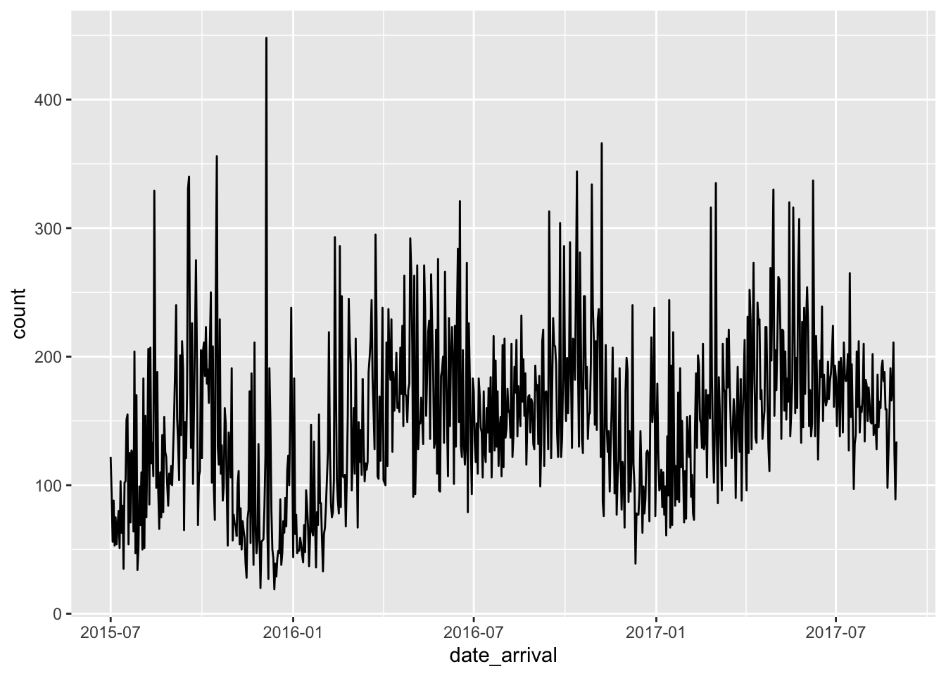
This doesn’t give us a lot of information. So lets try plotting a graph between cumulative bookings and date.
hotels_cumulbookings_bydate <- hotels_totalbookings_bydate %>%
mutate(cumulative=cumsum(count))
hotels_cumulbookings_bydateggplot(hotels_cumulbookings_bydate, aes(date_arrival, cumulative)) + geom_line()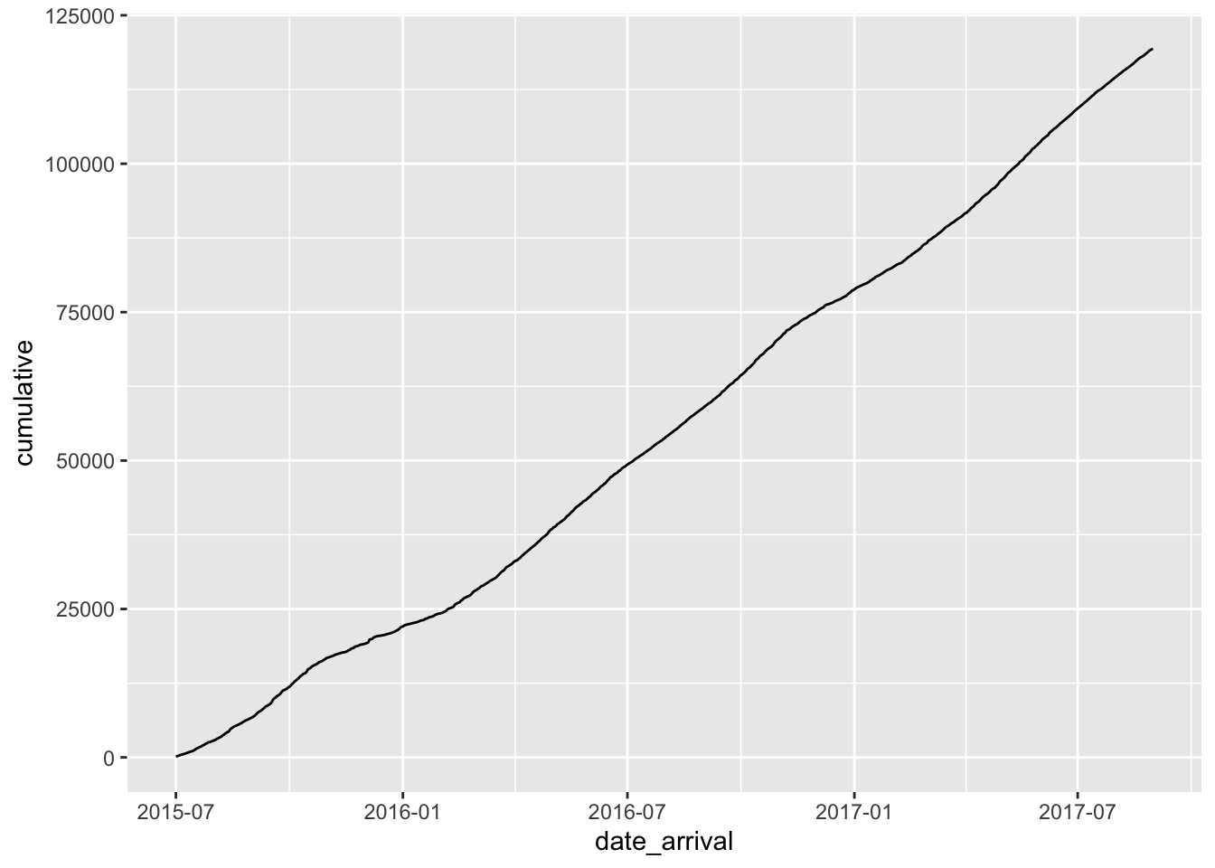
Now lets see which bookings by month
hotels_totalbookings_bymonth_pre <- hotel_mutated %>%
group_by(arrival_date_month) %>%
summarise(count = n())
hotels_totalbookings_bymonth <- hotels_totalbookings_bymonth_pre %>% mutate(
arrival_date_month = factor(arrival_date_month, levels = month.name)
) %>%
arrange(arrival_date_month)ggplot(hotels_totalbookings_bymonth, aes(arrival_date_month, count, group=1)) + geom_line() + geom_point()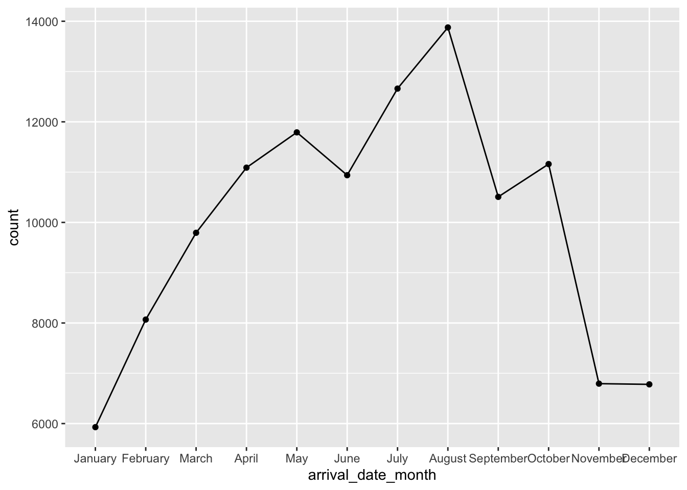
Now we also try and visualize which months bookings end up being cancelled the most. For this we will visualize the fraction of bookings that were cancelled for that month.
hotels_cancel_bymonth_pre <- hotel_mutated %>%
group_by(arrival_date_month) %>%
summarise(count = n(), cancelled=sum(is_canceled))
hotels_cancel_bymonth_pre <- hotels_cancel_bymonth_pre %>% mutate(fraction_cancelled = cancelled/count)
hotels_cancel_bymonth <- hotels_cancel_bymonth_pre %>% mutate(
arrival_date_month = factor(arrival_date_month, levels = month.name)
) %>%
arrange(arrival_date_month)
hotels_cancel_bymonthggplot(hotels_cancel_bymonth, aes(arrival_date_month, fraction_cancelled, group=1)) + geom_line() + geom_point()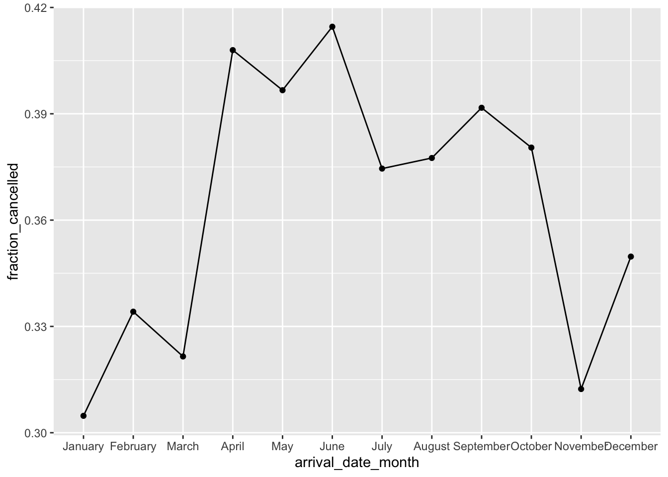
These graphs help hotels prepare for seasonal increase in bookings. There is a peak in bookings in August and hotels would want to scale up and down their resources accordingly. This would include staff, amenities etc. And since January sees the least number of visitors, it would make sense to do renovations during this time of the year.
Similarly we see that more than 40% bookings in April and June are cancelled, which means that the hotels can expect, the actual number of guests to be lower than the number of bookings made.
Visualizing Part-Whole Relationships
To visualize part-whole relationships we will try to visualise monthly sales for different types of hotels
hotels_totalbookings_bymonth_pre <- hotel_mutated %>%
group_by(arrival_date_month, hotel) %>%
summarise(count = n())
hotels_totalbookings_bymonth <- hotels_totalbookings_bymonth_pre %>% mutate(
arrival_date_month = factor(arrival_date_month, levels = month.name)
) %>%
arrange(arrival_date_month)ggplot(hotels_totalbookings_bymonth, aes(arrival_date_month, count, col=hotel, group=hotel)) + geom_line() + geom_point()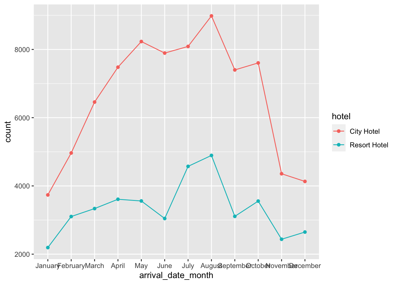
We can see that City hotels have more bookings than resort hotels. We also see that both hotel types follow similar trends. They have peaks during the same month.