Challenge 8: SNL Cast Analysis

Data Joining and Analysis on SNL Cast Information

library(tidyverse)
library(ggplot2)
library(lubridate)

knitr::opts_chunk$set(echo = TRUE, warning=FALSE, message=FALSE)

Read in data

SNL_actors <- read_csv("_data/snl_actors.csv")
SNL_casts <- read_csv("_data/snl_casts.csv")
SNL_seasons <- read_csv("_data/snl_seasons.csv")

Briefly describe the data

This dataset comprises three tables about the actors and seasons of SNL, a late-night comedy show which was once hosted by one of my favorite standup comedians, Norm Macdonald. The first table, actors, gives each actor’s name, gender, and cast type. The second table, casts, shows the relationship between an actor and the seasons in which they featured. It also includes how many episodes of the season they appeared in, as well as some statistical data. The third table, seasons, gives information on each season’s year, number of episodes, and episode ids. Casts describes the relationship between the two tables of entities, while actor and seasons include entries that reflect one entity.

Tidy Data (as needed)

The data needs no further preprocessing.

Join Data

To merge the datasets, we must consider the common keys. The casts and seasons datasets share the sid (season ID) column, whereas casts and actors share the aid (actor ID) column. We will first integrate the additional data from the actors dataset into the casts dataset, enabling us to analyze the genders of the actors.

# Create a new dataframe for 'cast' roles only from actors dataset
cast_actors <- SNL_actors %>%
       select(-url) %>%
       filter(type == "cast")  # Filters out all roles except 'cast'

# Count number of distinct actors in casts dataset
num_unique_actors <- SNL_casts %>%
      pull(aid) %>%
      unique() %>%
      length()  # Returns number of unique actors

# Merge cast_actors and casts datasets using 'aid' as the key
merged_casts <- merge(cast_actors, SNL_casts, by = "aid") %>%
        select(aid, gender, sid, featured, update_anchor)


print(num_unique_actors)

[1] 156

With this integrated data, we can now conduct analyses on the gender distribution throughout seasons as well as the gender representation among weekend update hosts.

# Join the datasets and create a new column 'gender_male'
gender_counts <- merged_casts %>%
    left_join(SNL_seasons, by = 'sid') %>%
    mutate(gender_male = gender == 'male') %>%
    select(sid, year, gender, gender_male, featured) %>%
    group_by(year, gender_male) %>%
    summarise(total_featured = sum(featured))

head(gender_counts, 3)

# A tibble: 3 × 3
# Groups:   year [2]
   year gender_male total_featured
  <dbl> <lgl>                <int>
1  1975 FALSE                    0
2  1975 TRUE                     0
3  1976 FALSE                    0

# Calculate the total counts per season
season_counts <- merged_casts %>%
    left_join(SNL_seasons, by = 'sid') %>%
    mutate(gender_male = gender == 'male') %>%
    select(sid, year, gender, gender_male, featured) %>%
    group_by(year) %>%
    summarise(total_featured = sum(featured))

head(season_counts, 3)

# A tibble: 3 × 2
   year total_featured
  <dbl>          <int>
1  1975              0
2  1976              0
3  1977              2

# Calculate the gender ratio
gender_ratio <- gender_counts %>%
    left_join(season_counts, by = 'year') %>%
    mutate(featured_ratio = total_featured.x / total_featured.y)

head(gender_ratio, 3)

# A tibble: 3 × 5
# Groups:   year [2]
   year gender_male total_featured.x total_featured.y featured_ratio
  <dbl> <lgl>                  <int>            <int>          <dbl>
1  1975 FALSE                      0                0            NaN
2  1975 TRUE                       0                0            NaN
3  1976 FALSE                      0                0            NaN

# Plot the data
ggplot(gender_ratio, aes(x = year, y = featured_ratio, col = gender_male)) +
    geom_bar(position = "stack", stat = "identity") +
    ggtitle('Ratio of Male to Non-Male Cast Members on SNL') +
    labs(x = 'Year', y = 'Ratio of Male to Non-Male', color = 'b')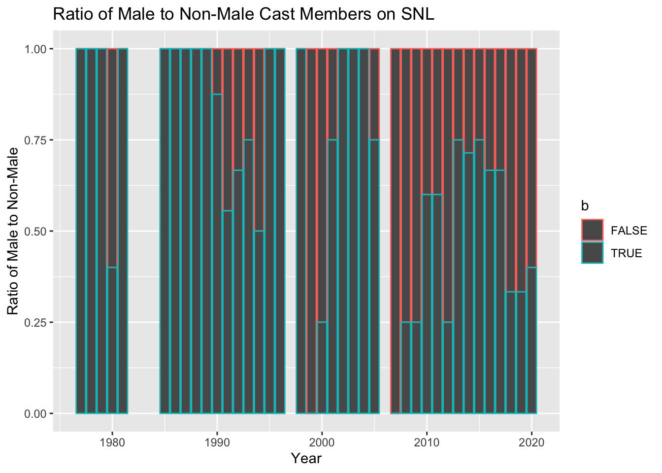

As we can see, the gender gap is shrinking year after year.