Challenge 8

challenge_8

Shaunak Padhye

snl

Joining Data

Author

Shaunak Padhye

Published

May 20, 2023

library(tidyverse)
library(ggplot2)

knitr::opts_chunk$set(echo = TRUE, warning=FALSE, message=FALSE)

Read in data

For this challenge I will be using the following dataset.

snl ⭐⭐⭐⭐⭐

snl_casts <- read_csv("_data/snl_casts.csv", skip = 1, col_names = c("aid", "sid", "featured", "cast_first_epid", "cast_last_epid", "update_anchor", "cast_n_epid", "season_fraction"))
  
snl_actors <- read_csv("_data/snl_actors.csv")
  
snl_seasons <- read_csv("_data/snl_seasons.csv", skip = 1, col_names = c("sid", "year", "seasons_first_epid", "seasons_last_epid", "seasons_n_epid"))

Briefly describe the data

This dataset contains three different dataframes:

snl_actors: The actors dataframe contains details of the cast of people who have appeared in SNL from 1975 to 2020.

snl_casts: The casts dataframe contains details of the cast for various seasons of SNL.

snl_seasons: The seasons dataframe contains details of each season from 1975 to 2020.

Tidy Data (as needed)

Lets look what dataframes we have.

head(snl_actors)

# A tibble: 6 × 4
  aid            url           type  gender 
  <chr>          <chr>         <chr> <chr>  
1 Kate McKinnon  /Cast/?KaMc   cast  female 
2 Alex Moffat    /Cast/?AlMo   cast  male   
3 Ego Nwodim     /Cast/?EgNw   cast  unknown
4 Chris Redd     /Cast/?ChRe   cast  male   
5 Kenan Thompson /Cast/?KeTh   cast  male   
6 Carey Mulligan /Guests/?3677 guest andy

We can remove the url column for our analysis.

snl_actors <- snl_actors %>% select(-url)
str(snl_actors)

tibble [2,306 × 3] (S3: tbl_df/tbl/data.frame)
 $ aid   : chr [1:2306] "Kate McKinnon" "Alex Moffat" "Ego Nwodim" "Chris Redd" ...
 $ type  : chr [1:2306] "cast" "cast" "cast" "cast" ...
 $ gender: chr [1:2306] "female" "male" "unknown" "male" ...

Lets look at the casts dataframe:

head(snl_casts)

# A tibble: 6 × 8
  aid      sid featured cast_first_epid cast_last_epid update_anchor cast_n_epid
  <chr>  <dbl> <lgl>              <dbl>          <dbl> <lgl>               <dbl>
1 A. Wh…    11 TRUE            19860222             NA FALSE                   8
2 A. Wh…    12 TRUE                  NA             NA FALSE                  20
3 A. Wh…    13 TRUE                  NA             NA FALSE                  13
4 A. Wh…    14 TRUE                  NA             NA FALSE                  20
5 A. Wh…    15 TRUE                  NA             NA FALSE                  20
6 A. Wh…    16 TRUE                  NA             NA FALSE                  20
# ℹ 1 more variable: season_fraction <dbl>

summary(snl_casts)

     aid                 sid         featured       cast_first_epid   
 Length:614         Min.   : 1.00   Mode :logical   Min.   :19770115  
 Class :character   1st Qu.:15.00   FALSE:451       1st Qu.:19801215  
 Mode  :character   Median :26.00   TRUE :163       Median :19901110  
                    Mean   :25.47                   Mean   :19909634  
                    3rd Qu.:37.00                   3rd Qu.:19957839  
                    Max.   :46.00                   Max.   :20141025  
                                                    NA's   :564       
 cast_last_epid     update_anchor    cast_n_epid    season_fraction  
 Min.   :19751011   Mode :logical   Min.   : 1.00   Min.   :0.04167  
 1st Qu.:19850112   FALSE:541       1st Qu.:19.00   1st Qu.:1.00000  
 Median :19950225   TRUE :73        Median :20.00   Median :1.00000  
 Mean   :19944038                   Mean   :18.73   Mean   :0.94827  
 3rd Qu.:20040117                   3rd Qu.:21.00   3rd Qu.:1.00000  
 Max.   :20140201                   Max.   :24.00   Max.   :1.00000  
 NA's   :597

Finally we take a look at the seasons data.

head(snl_seasons)

# A tibble: 6 × 5
    sid  year seasons_first_epid seasons_last_epid seasons_n_epid
  <dbl> <dbl>              <dbl>             <dbl>          <dbl>
1     1  1975           19751011          19760731             24
2     2  1976           19760918          19770521             22
3     3  1977           19770924          19780520             20
4     4  1978           19781007          19790526             20
5     5  1979           19791013          19800524             20
6     6  1980           19801115          19810411             13

summary(snl_seasons)

      sid             year      seasons_first_epid seasons_last_epid 
 Min.   : 1.00   Min.   :1975   Min.   :19751011   Min.   :19760731  
 1st Qu.:12.25   1st Qu.:1986   1st Qu.:19863512   1st Qu.:19872949  
 Median :23.50   Median :1998   Median :19975926   Median :19985512  
 Mean   :23.50   Mean   :1998   Mean   :19975965   Mean   :19985509  
 3rd Qu.:34.75   3rd Qu.:2009   3rd Qu.:20088423   3rd Qu.:20098015  
 Max.   :46.00   Max.   :2020   Max.   :20201003   Max.   :20210410  
 seasons_n_epid
 Min.   :12.0  
 1st Qu.:20.0  
 Median :20.0  
 Mean   :19.7  
 3rd Qu.:21.0  
 Max.   :24.0

Join Data

Now we will join the dataframes:

snl_castsseasons <- left_join(snl_casts, snl_seasons, by = "sid")

snl_data <- left_join(snl_castsseasons, snl_actors, "aid")

glimpse(snl_data)

Rows: 614
Columns: 14
$ aid                <chr> "A. Whitney Brown", "A. Whitney Brown", "A. Whitney…
$ sid                <dbl> 11, 12, 13, 14, 15, 16, 5, 39, 40, 41, 42, 45, 46, …
$ featured           <lgl> TRUE, TRUE, TRUE, TRUE, TRUE, TRUE, TRUE, TRUE, TRU…
$ cast_first_epid    <dbl> 19860222, NA, NA, NA, NA, NA, 19800409, 20140118, N…
$ cast_last_epid     <dbl> NA, NA, NA, NA, NA, NA, NA, NA, NA, NA, NA, NA, NA,…
$ update_anchor      <lgl> FALSE, FALSE, FALSE, FALSE, FALSE, FALSE, FALSE, FA…
$ cast_n_epid        <dbl> 8, 20, 13, 20, 20, 20, 5, 11, 21, 21, 21, 18, 17, 2…
$ season_fraction    <dbl> 0.4444444, 1.0000000, 1.0000000, 1.0000000, 1.00000…
$ year               <dbl> 1985, 1986, 1987, 1988, 1989, 1990, 1979, 2013, 201…
$ seasons_first_epid <dbl> 19851109, 19861011, 19871017, 19881008, 19890930, 1…
$ seasons_last_epid  <dbl> 19860524, 19870523, 19880227, 19890520, 19900519, 1…
$ seasons_n_epid     <dbl> 18, 20, 13, 20, 20, 20, 20, 21, 21, 21, 21, 18, 17,…
$ type               <chr> "cast", "cast", "cast", "cast", "cast", "cast", "ca…
$ gender             <chr> "male", "male", "male", "male", "male", "male", "ma…

Data Exploration

We can see the distribution of gender for the cast member who have been Weekend Update Anchors.

snl_data %>%
  filter(update_anchor == TRUE) %>%
  ggplot(aes(x = gender, fill = gender)) +
  geom_bar() +
  xlab("Gender") +
  ylab("Count") +
  ggtitle("Gender Distribution for Weekend Update") +
  scale_fill_brewer(palette = "Set1")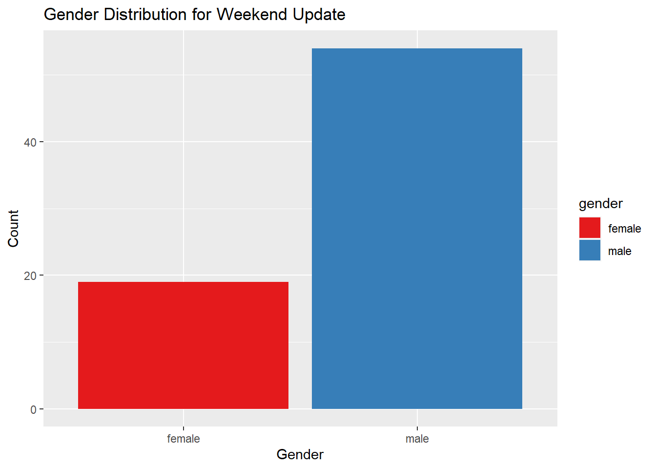

We can see from the above graph that SNL has cast more Male cast members over female cast members as the Weekend Update Anchor.

It will be interesting to see the gender distribution of cast members over the years.

snl_data %>%
  group_by(year, gender) %>%
  summarise(count = n()) %>%
  ggplot(aes(x = year, y = count, fill = gender)) +
  geom_bar(stat = "identity", position = "stack") +
  labs(x = "Year", y = "Count", fill = "Gender") +
  ggtitle("Gender Distribution by Year") +
  scale_fill_brewer(palette = "Set1") +
  theme_minimal()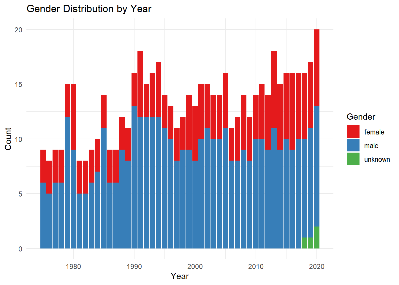

The percentage of female cast members has increased over the years. However, SNL still tends to cast more male actors than female.