This dataset shows AirBnB listings in NYC in 2019 with 48,895 rows (listings) and 17 columns (data for each listing). We see different types of observations including NYC neighborhood and neighborhood group, type of rental (entire home, private room, shared room), their prices, the minimum required number of nights, and number of guest reviews. Additionally we can see how many listing each host has on AirBnB, how many days a listing was available throughout 2019, and the date of the last guest review.
Read in the Data
I chose not to pivot this data because each listing was unique, even if a host had different listings, each had different price points, neighborhoods, room types, and names.
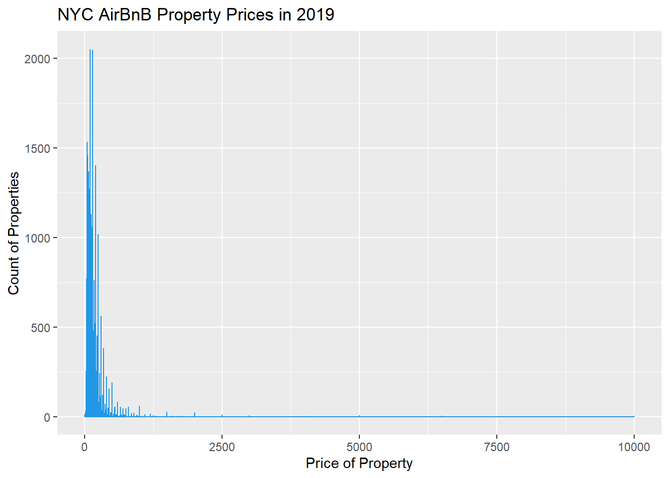
This graph here shows us that most of the listings are under $500 per night, though we see a few outliers past that point.
Code
# Price ggplotggplot(data, aes(price)) +geom_histogram(colour =4, fill ="white",binwidth = .15) +labs (title ="NYC AirBnB Property Prices in 2019", x ="Price of Property", y ="Count of Properties")
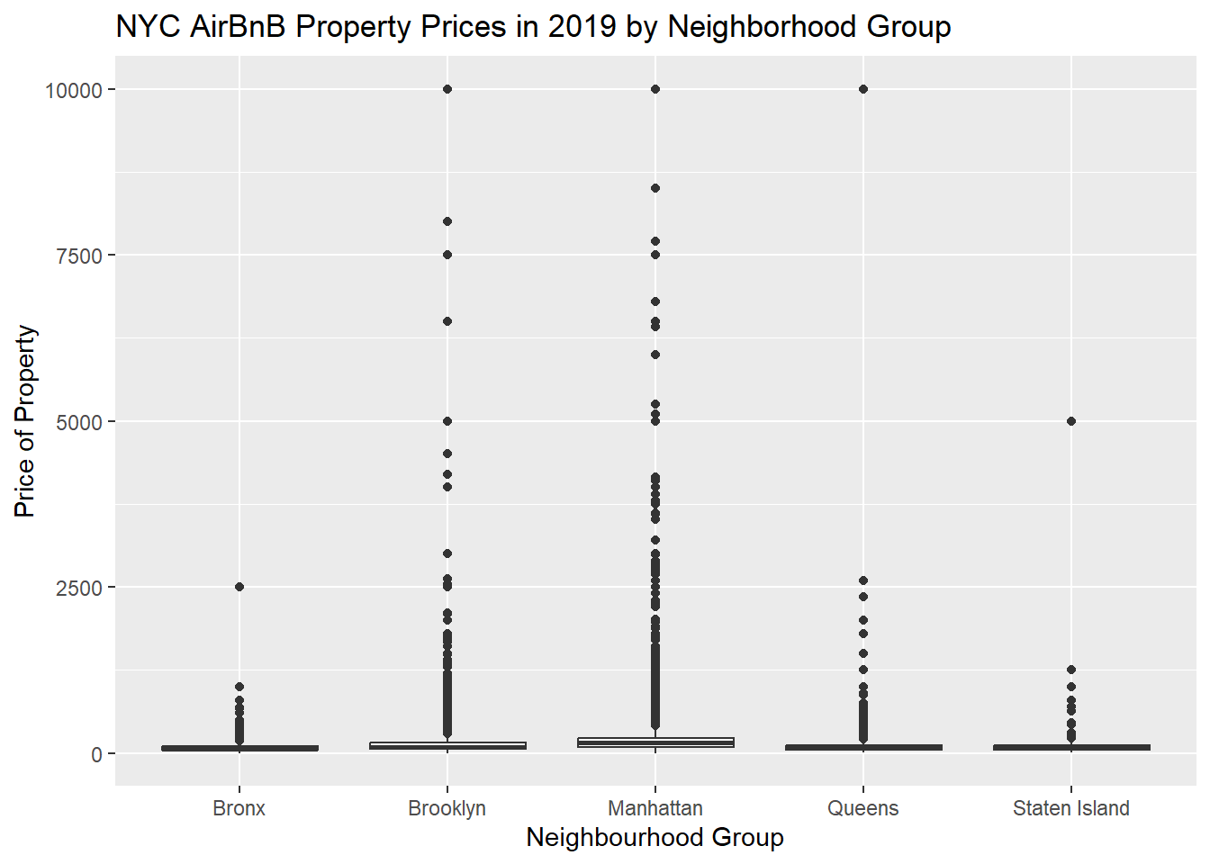
In a different angle we can see better that there are outliers in the price ranges, but the data are mostly represented in that under $500 price range.
Code
# Price ggplotggplot(data, aes(neighbourhood_group, price)) +geom_boxplot() +labs (title ="NYC AirBnB Property Prices in 2019 by Neighborhood Group", x ="Neighbourhood Group", y ="Price of Property")
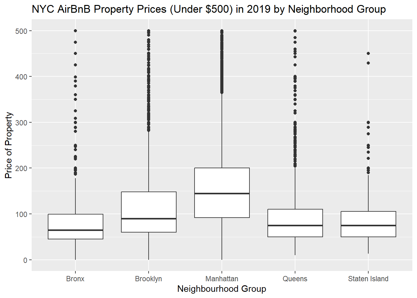
Let’s zoom in to that under $500 range.
Code
# If you wanted to just see the price for a listing under $500 this graph is more usefulggplot(data, aes(neighbourhood_group, price)) +geom_boxplot() +ylim(0, 500) +labs (title ="NYC AirBnB Property Prices (Under $500) in 2019 by Neighborhood Group", x ="Neighbourhood Group", y ="Price of Property")
Lets find the average price per room type and neighborhood group.
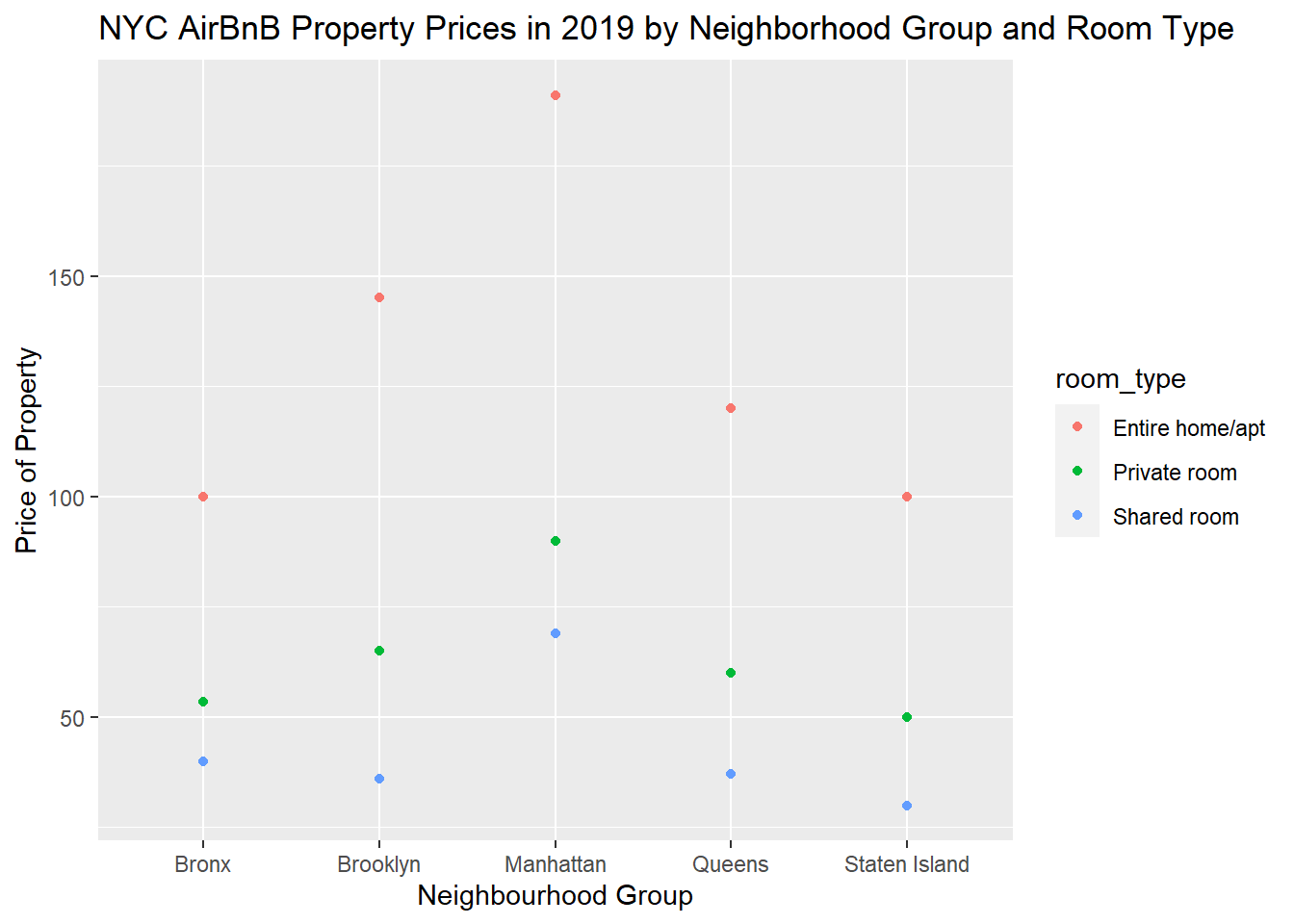
To no ones surprise the shared room’s are the least expensive of the three room types across neighborhoods. What’s interesting is that the average price for a shared room in Manhattan is more expensive than the average cost of a private room in any of the other neighborhood groups.
Code
# Price ggplotggplot(nm, aes(color = room_type, neighbourhood_group, price)) +geom_point() +labs(title="NYC AirBnB Property Prices in 2019 by Neighborhood Group and Room Type", x ="Neighbourhood Group", y ="Price of Property")
Maps - A trial and error
For Fun! - anyone want to add onto it? I’d be curious to see what others could come up with.
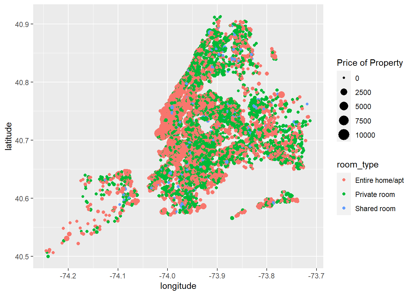
1st map
This first map Erico helped me with. Here we see the longitude and latitude points from the data mapped according to price and room type
Code
ggplot(data, aes(longitude, latitude, size = price, color = room_type), group = neighbourhood_group) +geom_point() +labs (size ="Price of Property")
2nd map
This second map I made of NYC but I couldn’t figure out how to plot the points from the data set
---title: "AirBnB New York 2019 Challenge 5"author: "Sue-Ellen Duffy"description: "Plotting Price per Neighbourhood Groups"date: "03/25/2023"format: html: toc: true code-fold: true code-copy: true code-tools: truecategories: - challenge_5 - Sue-Ellen Duffy - airbnb---```{r}#| label: setup#| warning: false#| message: falselibrary(tidyverse)library(readr)library(readxl)library(lubridate)library(ggplot2)library(dplyr)library(ggmap)library(maps)library(leaflet)library(broom)library(summarytools)library(hrbrthemes)library(plotly)knitr::opts_chunk$set(echo =TRUE, warning=FALSE, message=FALSE)```### AirBnB Listing Data in New York City 2019This dataset shows AirBnB listings in NYC in 2019 with 48,895 rows (listings) and 17 columns (data for each listing). We see different types of observations including NYC neighborhood and neighborhood group, type of rental (entire home, private room, shared room), their prices, the minimum required number of nights, and number of guest reviews. Additionally we can see how many listing each host has on AirBnB, how many days a listing was available throughout 2019, and the date of the last guest review.## Read in the DataI chose not to pivot this data because each listing was unique, even if a host had different listings, each had different price points, neighborhoods, room types, and names.```{r}data<-read.csv("_data/AB_NYC_2019.csv")tibble(data, 10)```The different data point for each listing:```{r}colnames(data)```## Univariate Graphs:# Price by Neighborhood GroupThis graph here shows us that most of the listings are under $500 per night, though we see a few outliers past that point.```{r}# Price ggplotggplot(data, aes(price)) +geom_histogram(colour =4, fill ="white",binwidth = .15) +labs (title ="NYC AirBnB Property Prices in 2019", x ="Price of Property", y ="Count of Properties")```In a different angle we can see better that there are outliers in the price ranges, but the data are mostly represented in that under $500 price range.```{r}# Price ggplotggplot(data, aes(neighbourhood_group, price)) +geom_boxplot() +labs (title ="NYC AirBnB Property Prices in 2019 by Neighborhood Group", x ="Neighbourhood Group", y ="Price of Property") ```Let's zoom in to that under $500 range.```{r}# If you wanted to just see the price for a listing under $500 this graph is more usefulggplot(data, aes(neighbourhood_group, price)) +geom_boxplot() +ylim(0, 500) +labs (title ="NYC AirBnB Property Prices (Under $500) in 2019 by Neighborhood Group", x ="Neighbourhood Group", y ="Price of Property") ```Lets find the average price per room type and neighborhood group.```{r}nm<-data%>%group_by(neighbourhood_group, room_type) %>%select(price) %>%summarize_all(median, na.rm =TRUE) %>%arrange(neighbourhood_group, price)nm```## Bivariate Graph: # Price by Neighborhood Group and Room TypeTo no ones surprise the shared room's are the least expensive of the three room types across neighborhoods. What's interesting is that the average price for a shared room in Manhattan is more expensive than the average cost of a private room in any of the other neighborhood groups.```{r}# Price ggplotggplot(nm, aes(color = room_type, neighbourhood_group, price)) +geom_point() +labs(title="NYC AirBnB Property Prices in 2019 by Neighborhood Group and Room Type", x ="Neighbourhood Group", y ="Price of Property")```## Maps - A trial and errorFor Fun! - anyone want to add onto it? I'd be curious to see what others could come up with.# 1st mapThis first map Erico helped me with. Here we see the longitude and latitude points from the data mapped according to price and room type```{r}ggplot(data, aes(longitude, latitude, size = price, color = room_type), group = neighbourhood_group) +geom_point() +labs (size ="Price of Property")```# 2nd mapThis second map I made of NYC but I couldn't figure out how to plot the points from the data set```{r}leaflet() %>%addTiles() %>%setView(-74.00, 40.71, zoom =12) %>%addProviderTiles("CartoDB.Positron")```# 3rd mapThis third map is my attempt of plotting in some data... clearly it didn't work```{r}entire_home <-data%>%filter(room_type =="Entire home/apt")private_room <-data%>%filter(room_type =="Private room")shared_room <- data%>%filter(room_type =="Shared room")``````{r}#from https://r-graph-gallery.com/242-use-leaflet-control-widget.htmldata_entire_home <-data.frame(LONG=-74.00+rnorm(17), LAT=40+rnorm(17), PLACE=paste(entire_home,seq(1,17)))data_private_room <-data.frame(LONG=-74.00+rnorm(17), LAT=40+rnorm(17), PLACE=paste(private_room,seq(1,17)))data_shared_room <-data.frame(LONG=-74.00+rnorm(17), LAT=40+rnorm(17), PLACE=paste(shared_room,seq(1,17)))m <-leaflet() %>%setView(lng=-74.00, lat=40, zoom=12 ) %>%addProviderTiles("CartoDB.Positron") %>%addCircleMarkers(data=data_entire_home, lng=~LONG , lat=~LAT, radius=8 , color="black",fillColor="red", stroke =TRUE, fillOpacity =0.8, group="Red") %>%addCircleMarkers(data=data_private_room, lng=~LONG , lat=~LAT, radius=8 , color="black",fillColor="blue", stroke =TRUE, fillOpacity =0.8, group="Blue") %>%addCircleMarkers(data=data_shared_room, lng=~LONG , lat=~LAT, radius=8 , color="black",fillColor="green", stroke =TRUE, fillOpacity =0.8, group="Blue") %>%addLayersControl(overlayGroups =c("Entire Home","Private Room","Shared Room") , baseGroups =c("background 1","background 2"),options =layersControlOptions(collapsed =FALSE))m```