The dataset was retrieved from the Massachusetts Department of Transportation data extraction service. I requested publicly available crash data for Boston municipality for the specific years of 2012-2022 and received a CSV file. Car crashes are reported to the Registry of Motor Vehicle and from there the Department of Transportation makes data available to the public.
This dataset includes 45,980 individual crashes in Boston from 2012-2022 which are represented by each row in the dataset. The dataset includes crash information including date, time, weather and lighting conditions and the severity of each crash. In regards to location, the dataset includes the travel direction of the vehicles, proximity to certain landmarks such as an exit or roadway intersection and the coordinates (latitude and longitude) of the crash point.
Post-pandemic car ownership and commuting by car has increased in an astonishing way - not to help the matter, train commutes are slower than ever. This dataset cannot delve deep enough to understand the scope of this transit issue and traffic data is not publicly available. This dataset will at least allow me to analyze city crashes that may yield some understanding about the implications of an increase in car commuting to the city. In a 2022 report by Inrix, Boston ranked 4th on the Global Traffic Scorecard, but not in the good way.
Questions
Are crashes in Boston increasing overtime? What type if any are increasing over time?
Are there any correlations to time of day, date, or road surface conditions that implicate a higher severity of crash and or more crashes overall?
How did the pandemic affect Boston crashes?
Data Description
Crash Date - Date occurrence of crash (year, month, and day)
Crash Time - Time occurrence of crash (hour, min, and sec)
Crash Severity - Indicates the severity of a crash based on the most severe injury to any person based on 3 levels - Fatal injury, Non-fatal injury, Property damage only (no injury) - and either Unknown or Not Reported
Maximum Injury Severity Reported - Reported injury if both fatal and non-fatal will be categorized “Fatal injury” as it is the most severe reported injury
Non_Motorist_Type - The type of non-motorist
Crash Hour - [added for analysis] Time occurrence of crash (hour only)
Crash Timegroup - [added for analysis] Time occurrence of crash (defined by time intervals: (Overnight = 2AM-5:59AM; Morning = 6AM-9:59AM; Midday = 10AM-1:59PM; Afternoon = 2PM-5:59PM; Evening = 6PM-9:59PM; Late Night = 10PM-1:59AM)
Crash Count - [added for analysis] Number of crash occurrences per day
Crash Countgroup - [added for analysis] Number of crash occurrences per day (defined by group intervals: (1-5, 6-10, 11-15, 16-20, 21-25, 26-30, 31-35, 36-40)
Handling Unknown, Not Reported, NA or Missing data
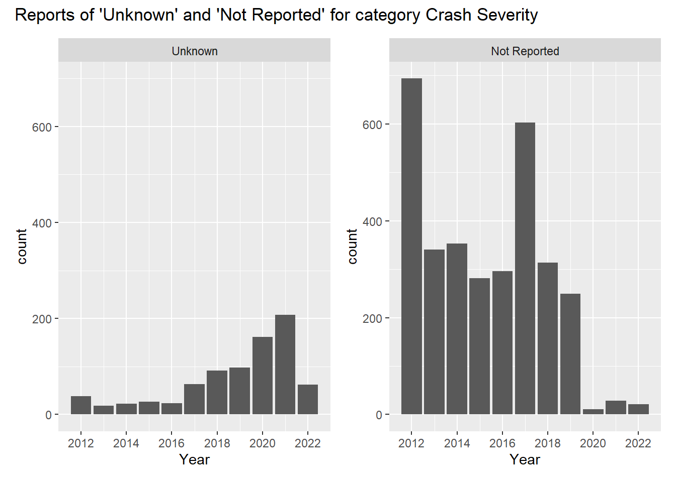
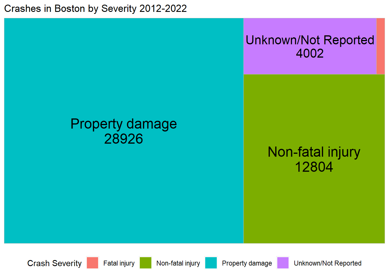
Unknown/Not Reported Data: There were 45,980 crashes reported from 2012 to 2022. Of those crashes 4,002 (8.7%) were reported with a Crash Severity of “Unknown” or “Not Reported” the majority are reported as resulting in property damage only with no injuries reported. Ranking second is non-fatal injuries, and finally a small portion are rated as fatal injuries.
For the purpose of this report, and for the category of “Crash Severity” only, I have combined these into “Unknown/Not Reported”.
Why are some crashes reported as Unknown or Not Reported? Possibilities include: + internal clerical errors
reports must be completed within 5 days of crash (leading to rushed answers)
decision fatigue from having to fill out the report alone post accident
data missing due to personal choice in managing insurance claims
Unknown/Not Reported Over Time: The category “Unknown” was used more so in later years, with a peak in 2021. Whereas “Not Reported” had peaks in 2012 and 2017 and very low numbers in 2020-2022.
Unknown/Not Reported Data Inconsistencies: Crashes that were reported under Crash Severity as being “Unknown” or “Not Reported” had 50 inconsistently reported injuries in another column of the data. All 50 reporting inconsistencies occurred between May 2018 and October 2019:
Crash Severity “Not Reported” has 42 reports of maximum injury reports across 6 categories that suggest a possible injury.
Crash Severity “Unknown” has 7 reports of non-fatal injury as either “Non-incapacitating” or “Possible” and 1 report of “No apparent injury”.
Road Surface Condition has an NA count of n=368. For the purpose of this report I am considering this sort of NA to be comparable with “Not Reported” or “Unknown” and leave the data in the dataset as I am only looking at a few indicators of Road Surface Condition and not analyzing it in depth.
Manner of Collision also has an NA count of n=5. I will leave that data alone as well.
Overview of Crash Data in Boston 2012-2022
Code
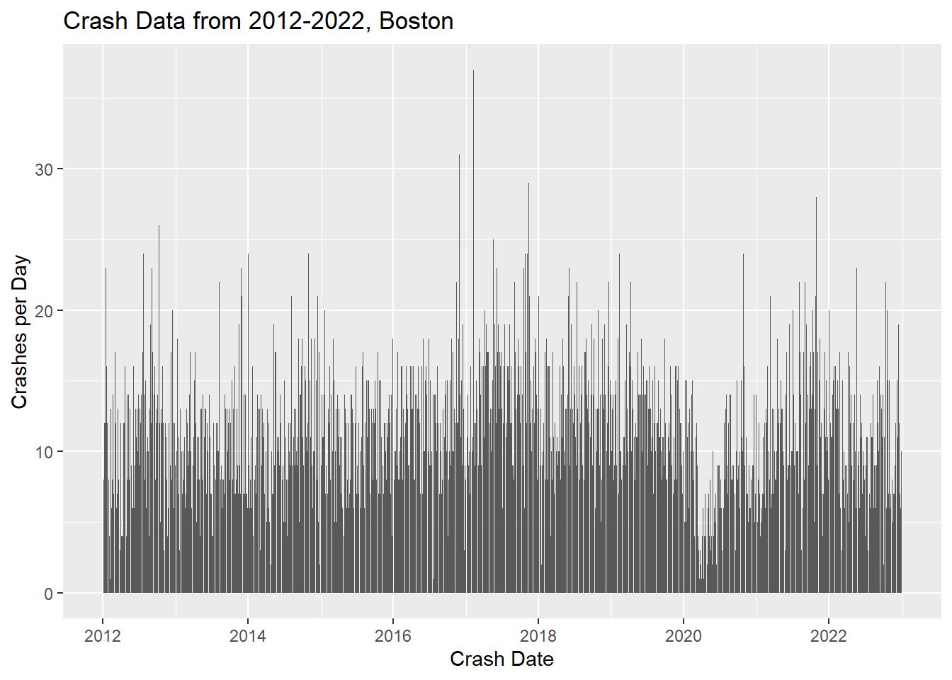
ggplot(mydata, aes(Crash_Date, stat="count")) +geom_bar() +labs(x="Crash Date", y="Crashes per Day", title ="Crash Data from 2012-2022, Boston")
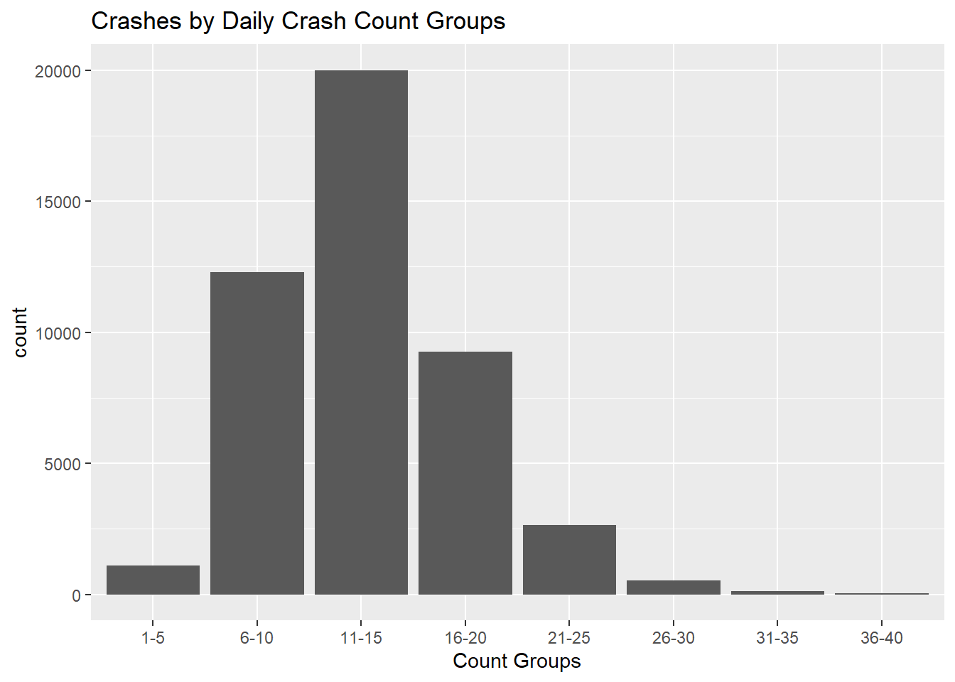
By viewing daily crash counts in intervals of 5 we can see that on most days there are 11-15 crashes in Boston, with some days having 6-10 or 16-20 crashes.
Very few days have 5 or less crashes.
Code
ggplot(mydata, aes(Crash_Countgroup, stat="count")) +geom_bar() +scale_x_discrete(limit =position_Countgroup) +labs(title ="Crashes by Daily Crash Count Groups", x ="Count Groups")
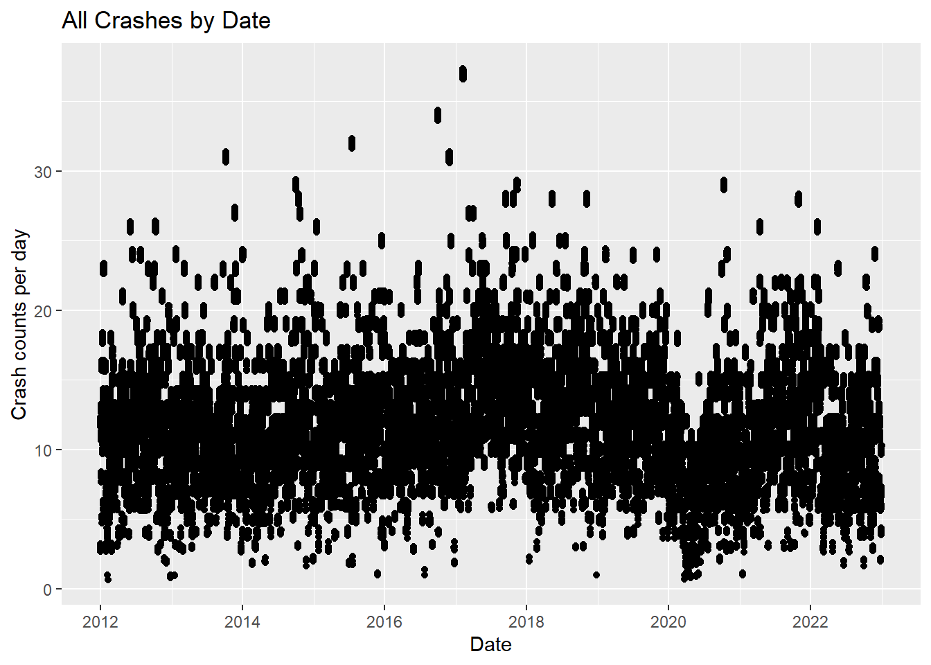
The following graph shows the density of crashes with crash counts per day. As opposed to the bargraph charting all crashes by total counts in the Overview, this graph lets us see outliers not only in the top portion of the graph with the most counts, but also in the lowest counts. We can now see the pockets of time when there were, for instance, more than 6 crashes per day everyday, like in 2017, or the time when in 2020 there were many instances of having only a 1-3 crashes per day.
Code
ggplot(mydata, aes(Crash_Date, y=Crash_Count, group = Crash_Severity)) +geom_point() +geom_jitter() +labs(title ="All Crashes by Date", y ="Crash counts per day", x ="Date")
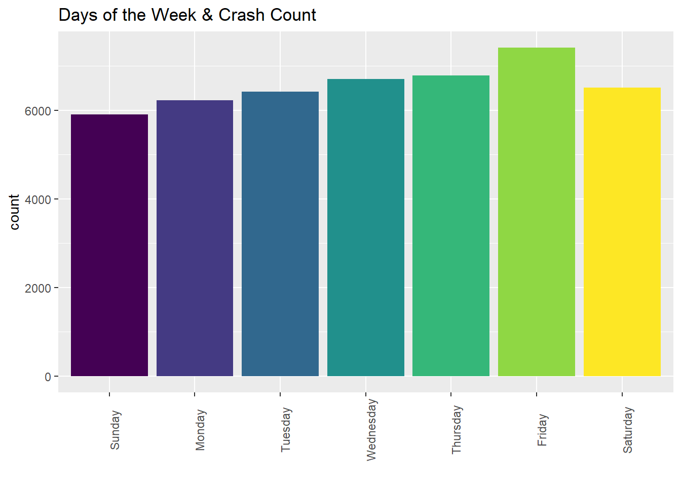
Boston saw the most crashes on Fridays (2012-2022).
Code
mydata %>%ggplot(aes(Weekday, fill = Weekday)) +geom_bar( stat ="count") +theme(axis.text.x =element_text(angle =90)) +theme(legend.position ="none") +labs(title ="Days of the Week & Crash Count", x ="")
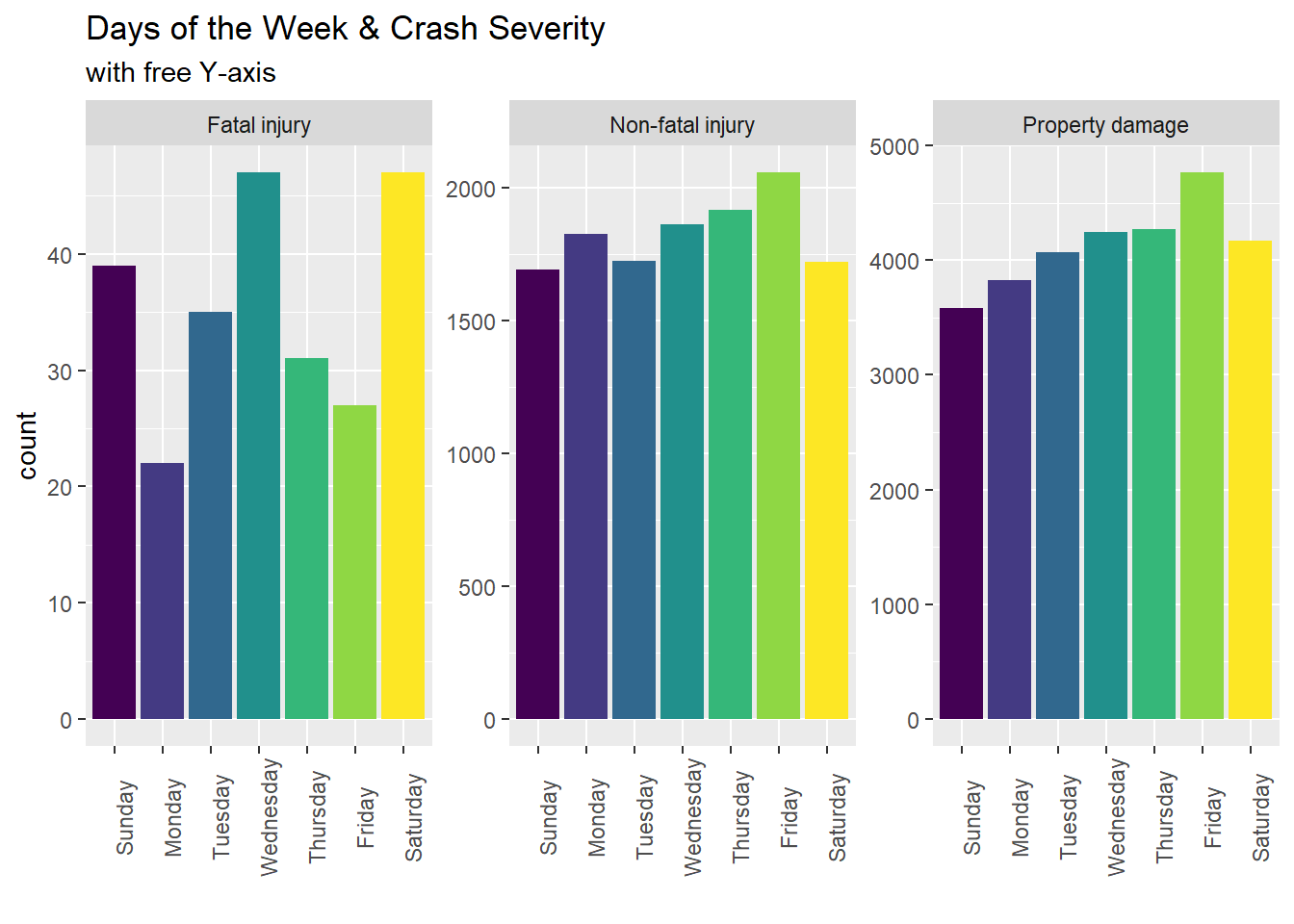
When subsetted for Crash Severity, however Boston sees the most fatal accidents on Wednesday and Saturday. (The following graph shows Crash Severity: Fatal injury, Non-fatal injury, and Property damage. It does not include Unknown/Not Reported)
Code
mydata %>%filter(Crash_Severity !="Unknown/Not Reported") %>%ggplot(aes(Weekday, fill = Weekday)) +geom_bar( stat ="count") +facet_wrap ( ~ Crash_Severity, scales ="free_y") +theme(axis.text.x =element_text(angle =90)) +theme(legend.position ="none") +labs(title ="Days of the Week & Crash Severity", subtitle ="with free Y-axis", x ="")
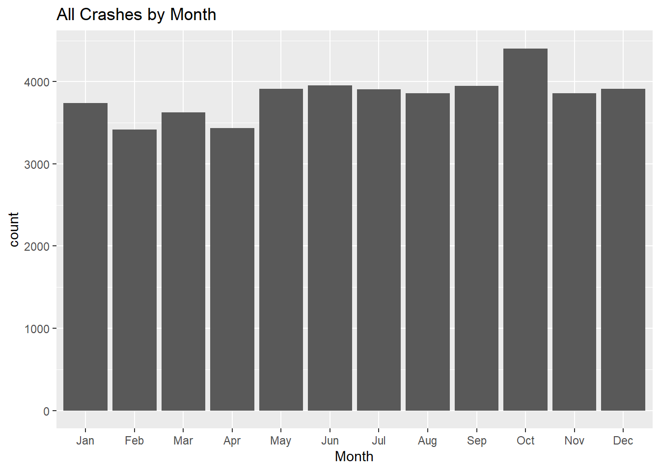
October is the month with the most crashes and the highest average crash rate in Boston (2012-2022), averaging 15 crashes per day.
Buckle up, this tab has a longer analysis section.
Code
#Crash Count per Day by Monthmydatamonthsum <- mydata %>%group_by(Month) %>%summarize("min"=min(Crash_Count, na.rm =TRUE),"max"=max(Crash_Count, na.rm =TRUE),"mean"=mean(Crash_Count, na.rm =TRUE), "median"=median(Crash_Count, na.rm =TRUE),"standard_deviation"=sd(Crash_Count, na.rm =TRUE))%>%arrange(Month)mydatamonthsum %>%kbl(caption ="Crash Statistic by Month") %>%kable_classic() %>%row_spec(10, bold = T, color ="black", background ="orange")
Crash Statistic by Month
Month
min
max
mean
median
standard_deviation
Jan
1
26
12.72292
12
4.561773
Feb
1
37
12.60901
12
4.740875
Mar
1
27
12.38372
12
4.475690
Apr
1
26
12.23283
12
4.174287
May
1
28
13.22847
13
4.504422
Jun
1
26
13.50594
13
4.349584
Jul
1
32
13.16479
13
4.600828
Aug
3
22
12.46228
12
3.640509
Sep
2
28
13.42582
13
4.272076
Oct
2
34
15.13079
14
5.736485
Nov
1
31
13.87772
13
5.403354
Dec
1
25
13.28206
13
4.378017
Code
ggplot(mydata, aes(Month, stat="count")) +geom_bar() +labs(title ="All Crashes by Month")
What could we learn about October?
+ Do road conditions have something to do with the increase in accidents?

+ Are there different types of accidents in October?

+ Is it all happening around Halloween?
Road Surface Conditions
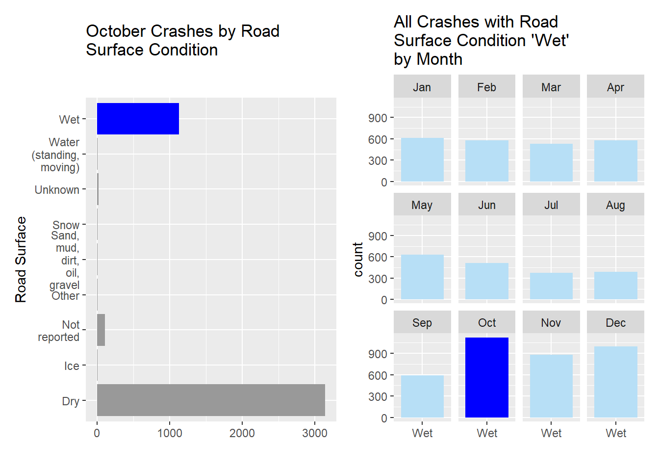
When we subset the data for October by road surface condition we see that “dry” is the predominant condition, however we see “Wet” with a large portion of data as well.
Code
wet1 <- mydata %>%filter(Month =="Oct") %>%ggplot(., aes(Road_Surface_Condition, stat ="count", fill = (Road_Surface_Condition =="Wet"))) +geom_bar() +coord_flip() +labs(x ="Road Surface", y ="", title =str_wrap("October Crashes by Road Surface Condition", width =25)) +scale_x_discrete(labels =function(x) str_wrap(x, width =5))+theme(legend.position ="none") +scale_fill_manual(values=c( "#999999", "#0000FF"))wet2 <- mydata %>%filter(Road_Surface_Condition =="Wet") %>%ggplot(., aes(Road_Surface_Condition, stat ="count", fill = Month)) +geom_bar() +facet_wrap( ~ Month,) +labs(x ="", title =str_wrap("All Crashes with Road Surface Condition 'Wet' by Month", width =25)) +theme(legend.position ="none") +scale_fill_manual(values=c("#B7DFF6", "#B7DFF6", "#B7DFF6", "#B7DFF6", "#B7DFF6", "#B7DFF6", "#B7DFF6", "#B7DFF6", "#B7DFF6", "#0000FF", "#B7DFF6", "#B7DFF6"))wet1 + wet2
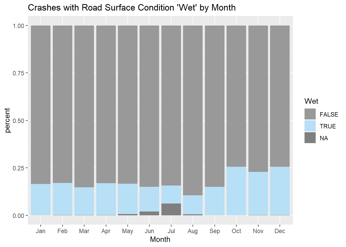
While October has the most crashes with “Wet” road surface conditions reported, October also has the most crashes overall. In order to understand whether this road surface condition “Wet” was a factor in making October the month with the highest crash rating, I looked at the percentages of crashes in each month that occurred under “Wet” road surface conditions. October and December both have 25% of crashes (per their respective months) with “Wet” road surface conditions reported.
Code
mydata %>%ggplot(., aes(Month, stat ="count", fill = (Road_Surface_Condition =="Wet"))) +geom_bar(position ="fill") +labs(title ="Crashes with Road Surface Condition 'Wet' by Month", y ="percent", x ="Month", fill ="Wet") +scale_fill_manual(values=c("#999999", "#B7DFF6", "#999999"))
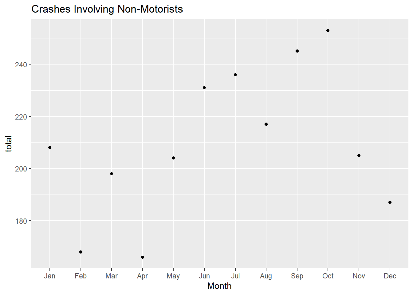
October is the month with the most instances of Non-motorist type involvement in crashes with 253 reports.
Code
nm<-mydata%>%select(Month, Non_Motorist_Type)%>%group_by(Month,Non_Motorist_Type)%>%count()nm<-pivot_wider(nm,names_from=Non_Motorist_Type,values_from = n)nm <-mutate_all(nm, ~replace_na(.,0))nm <- nm %>%select(., -"NA")nm <-nm %>%mutate(total =sum(c_across("P1: Pedestrian":"P2: Cyclist / P3: Other / P4: Other"))) %>%ungroup() nm <- nm %>%mutate(across("P1: Pedestrian":"P2: Cyclist / P3: Other / P4: Other" , ~ ./ total)) %>%mutate(across("P1: Pedestrian":"P2: Cyclist / P3: Other / P4: Other", ~ .*100))#total instances of crashes with Non-Motorists reported by Monthggplot(nm, aes(x=Month, y = total)) +geom_point() +labs(title ="Crashes Involving Non-Motorists")
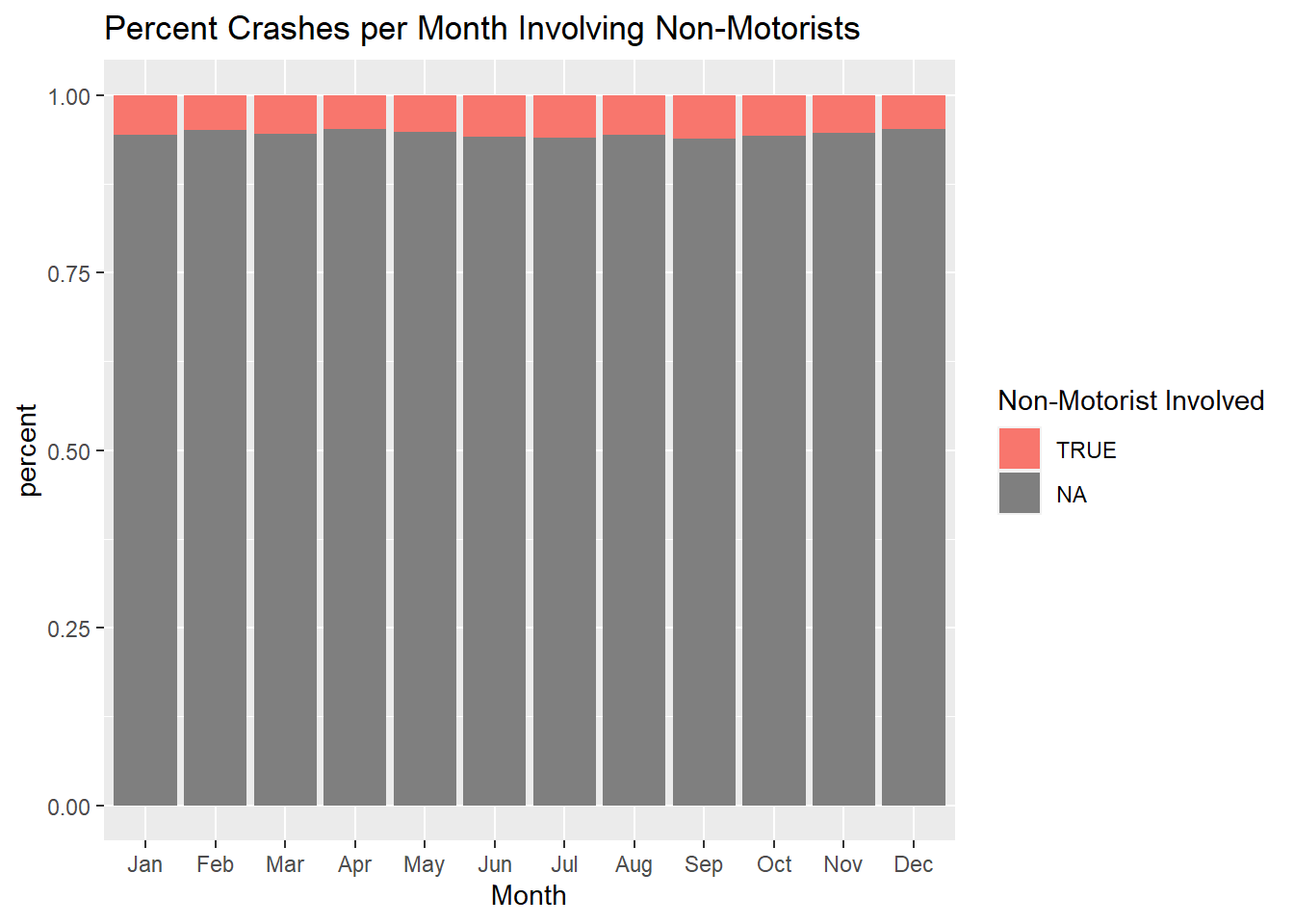
However proportional to the total number of crashes per Month, we see that July and September have the highest % of crashes involving non-motorist types.
Code
mydata %>%ggplot(., aes(Month, stat ="count", fill = (Non_Motorist_Type !="NA"))) +geom_bar(position ="fill") +labs(title ="Percent Crashes per Month Involving Non-Motorists", y ="percent", fill ="Non-Motorist Involved")
Crash Severity
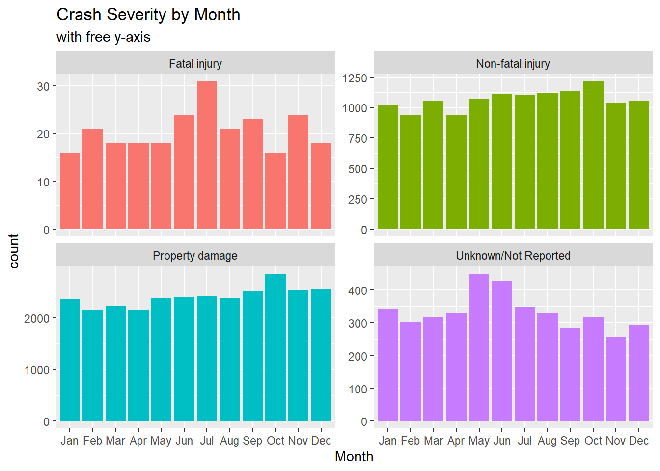
Let’s look at how each crash severity rating factors into this month analysis.
We can now see that the month with the highest Fatal injury is reported in July, with dips in spring, winter, and October while Non-fatal injuries and Property damage peak in October. The peak for Unknown/Not Reported crashes is in May and June.
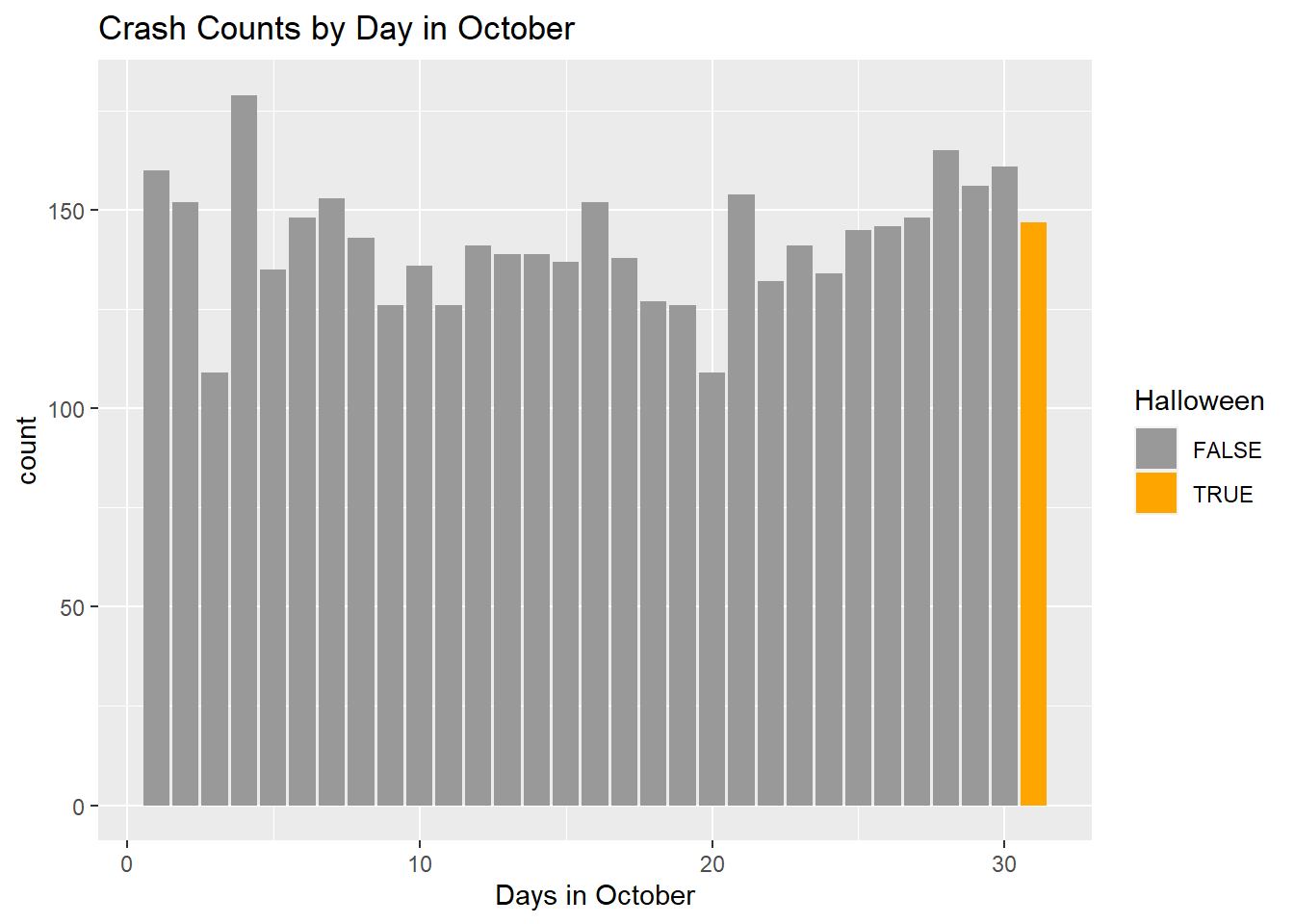
October 4th has the most counts of crashes in the month, which happens to be National Taco Day and World Animal Day.
Code
mydata %>%filter(Month =="Oct") %>%ggplot(., aes(x =Day, stat ="count", fill = (Day =="31"))) +geom_bar() +scale_fill_manual(values=c("#999999", "orange"))+labs(title ="Crash Counts by Day in October", x ="Days in October", fill ="Halloween")
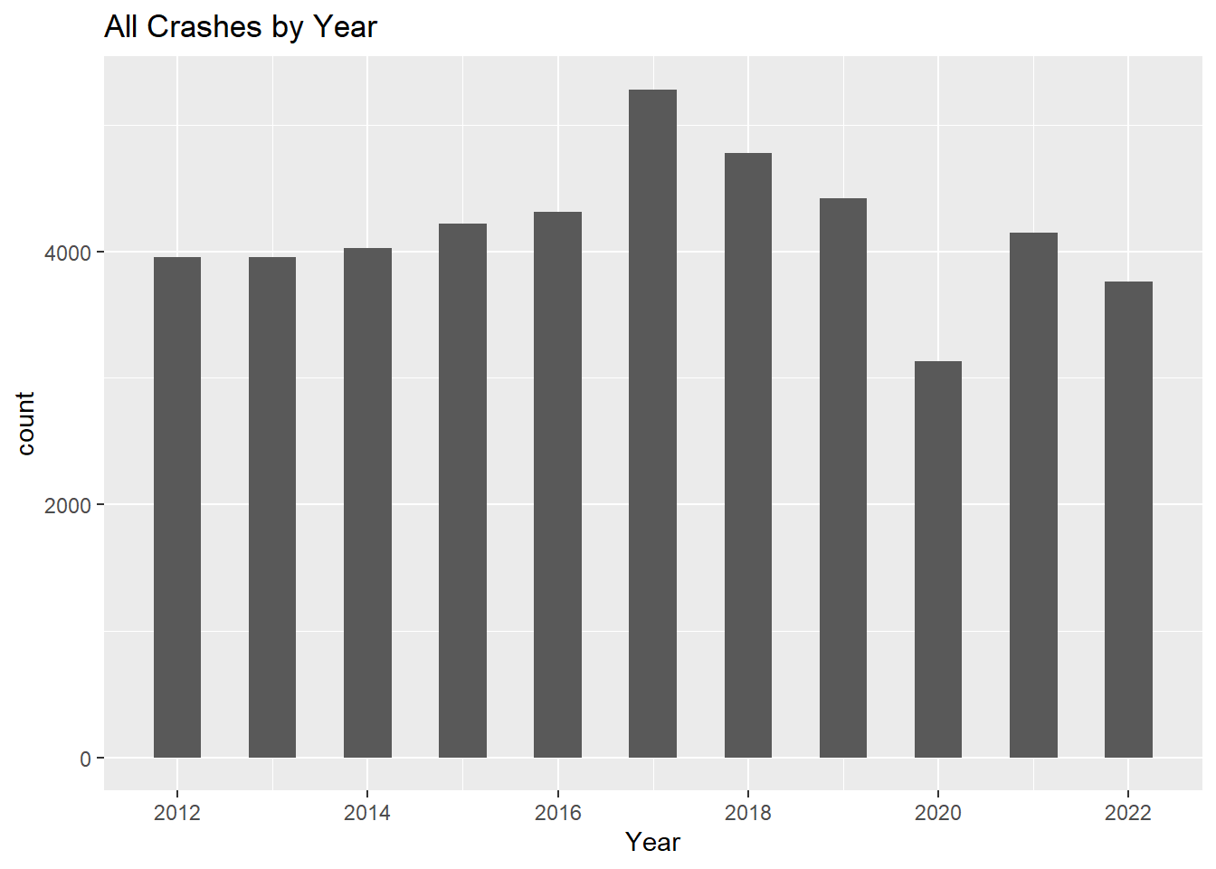
2017 was the year with the most crashes in Boston (2012-2022).
Code
#Crash Count per Day by Yearmydatasum <- mydata %>%group_by(Year) %>%summarize("min"=min(Crash_Count, na.rm =TRUE),"max"=max(Crash_Count, na.rm =TRUE),"mean"=mean(Crash_Count, na.rm =TRUE), "median"=median(Crash_Count, na.rm =TRUE),"standard deviation"=sd(Crash_Count, na.rm =TRUE)) %>%arrange(Year)mydatasum %>%kbl(caption ="Crash Statistic by Year") %>%kable_classic() %>%row_spec(6, bold = T)
Crash Statistic by Year
Year
min
max
mean
median
standard deviation
2012
1
26
12.52212
12
4.407276
2013
1
31
12.44976
12
4.607583
2014
2
29
12.79468
12
4.780628
2015
1
32
13.18238
13
4.592712
2016
1
34
13.21089
13
4.439938
2017
6
37
15.78167
15
4.718541
2018
1
28
14.61683
14
4.435525
2019
4
24
13.34472
13
3.918186
2020
1
29
10.59297
10
4.454502
2021
1
28
13.10707
13
4.704753
2022
2
26
11.97473
12
4.372023
The data shows 2017 as a peak with a sharp drop off in 2020 (due to the pandemic and reduced traffic flow) then a climb back up in 2021 almost matching crash reports from 2019. Of course this data shows that post-pandemic rates of car crashes have gone back up, but it is not as high as crashes in 2017.
Code
ggplot(mydata, aes(year(Crash_Date))) +geom_histogram(binwidth = .50) +scale_x_continuous(breaks=pretty_breaks()) +labs(title ="All Crashes by Year", x ="Year",)
What happened in 2017 and were these crashes somehow different from crashes in other years?
Road Surface Conditions
2017 had the most incidents of crash where “Ice” was the indicated road surface condition. Not the most significant data point considering its low n(79) but interesting none the less.
Code
datayear <- mydatadatayear =table(datayear$Year, datayear$Road_Surface_Condition) datayear %>%kbl(caption ="Road Conditions of Crashes (2012-2022) by Year" ) %>%kable_classic() %>%column_spec(3, bold = T) %>%row_spec(6, color ="black", background ="#B7DFF6")
Road Conditions of Crashes (2012-2022) by Year
Dry
Ice
Not reported
Other
Sand, mud, dirt, oil, gravel
Slush
Snow
Unknown
Water (standing, moving)
Wet
2012
2814
13
240
3
11
6
28
17
5
817
2013
2912
25
196
4
12
14
90
3
1
694
2014
2878
28
239
3
10
10
71
10
6
768
2015
3188
47
140
3
14
24
133
9
2
660
2016
3451
15
103
4
2
5
69
9
2
655
2017
4133
79
79
5
6
10
99
50
5
813
2018
3737
30
42
3
3
6
61
39
4
849
2019
3221
33
20
1
9
7
88
14
4
663
2020
2460
16
24
4
2
5
37
10
4
568
2021
3295
6
46
1
1
5
47
9
4
733
2022
3006
47
38
3
6
10
66
6
1
576
Number of Vehicles Involved
2017 had the most 2 car accidents and had 1 instance each of a 12 car and 18 car crash. Both of these high number crashes were in fact Ice related.
While a crash may involve multiple cars, the counts recorded throughout the data and this analysis are on individual crashes (regardless of how many cars are involved in the crash)
Code
#Year and Number of Vehiclesdatayearvehicles <- mydatadatayearvehicles =table(datayearvehicles$Year, datayearvehicles$Number_of_Vehicles) datayearvehicles %>%kbl(caption ="Number of Vehicles Involved in Crashes (2012-2022) by Year" ) %>%kable_classic() %>%column_spec(3:4, bold = T) %>%row_spec(6, color ="black", background ="#B7DFF6")
Number of Vehicles Involved in Crashes (2012-2022) by Year
0
1
2
3
4
5
6
7
8
9
10
11
12
18
2012
1
1109
2366
372
73
27
4
2
0
1
0
0
0
0
2013
0
1047
2354
422
98
19
8
0
2
0
0
1
0
0
2014
0
1059
2383
463
92
22
3
0
0
1
0
0
0
0
2015
0
981
2637
452
127
20
5
0
0
0
0
0
0
0
2016
0
933
2726
501
125
22
5
2
0
0
1
0
0
0
2017
0
1131
3383
581
140
32
9
1
1
1
0
0
1
1
2018
0
951
3121
526
143
19
9
4
2
1
0
0
0
0
2019
0
825
2914
530
108
30
10
4
0
0
0
0
0
0
2020
0
860
1829
331
77
23
6
3
0
1
0
0
0
0
2021
0
948
2567
484
106
28
10
3
0
0
1
0
0
0
2022
0
855
2367
423
81
26
4
1
0
2
0
0
0
0
Non-Motorists Involved
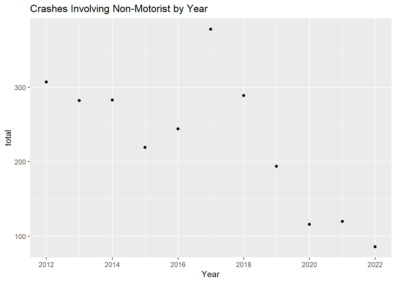
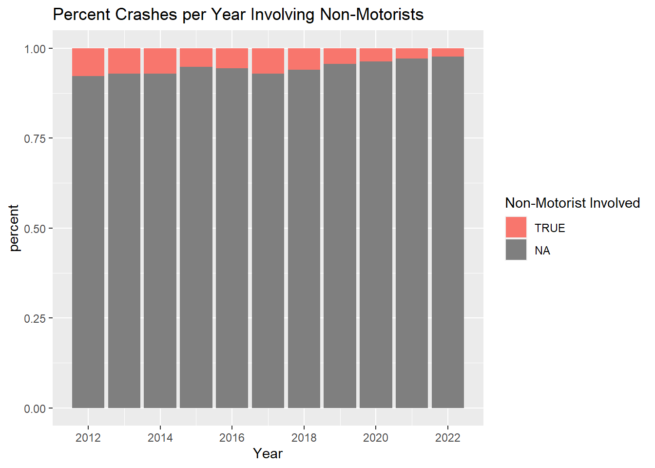
2017 is the year with the most crashes involving Non-Motorists with 378 crashes.
However, again, while it has the most instances of Non-motorist involvement, 2017 has just about the same percent of crashes as 2012 and 2013, with around 7% of all crashes in each of those years involving non-motorists
Code
mydata %>%ggplot(., aes(Year, stat ="count", fill = (Non_Motorist_Type !="NA"))) +geom_bar(position ="fill") +scale_x_continuous(breaks=pretty_breaks()) +labs(title ="Percent Crashes per Year Involving Non-Motorists", y ="percent", fill ="Non-Motorist Involved")
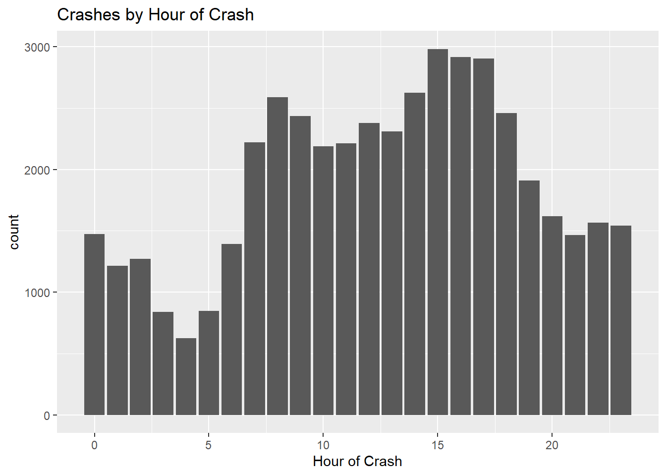
Most crashes occur in the afternoon, between 3pm and 5pm, in Boston (2012-2022).
Code
ggplot(mydata, aes(Crash_Hour)) +geom_histogram(stat="count") +labs(title ="Crashes by Hour of Crash", x ="Hour of Crash")
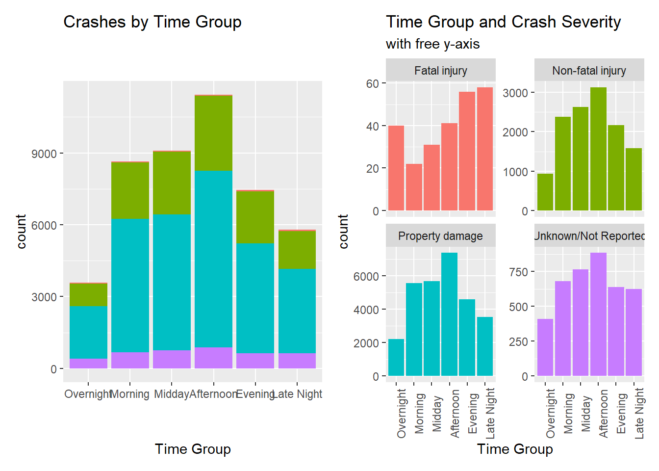
While Non-fatal, Property damage, Unknown/Not Reported all follow the same pattern of peaks in the afternoon, crashes resulting in Fatal injury peak at late night.
Time occurrence of crash (defined by time intervals: (Overnight = 2AM-5:59AM; Morning = 6AM-9:59AM; Midday = 10AM-1:59PM; Afternoon = 2PM-5:59PM; Evening = 6PM-9:59PM; Late Night = 10PM-1:59AM)
Code
tgroup <-ggplot(mydata, aes(Crash_Timegroup, stat="count", fill = Crash_Severity)) +geom_bar() +scale_x_discrete(limits = positions) +labs(title ="Crashes by Time Group", x ="Time Group", fill ="Crash Severity") +theme(legend.position ="none")csgroup <-ggplot(mydata, aes(Crash_Timegroup, stat="count", fill = Crash_Severity)) +geom_bar() +facet_wrap ( ~ Crash_Severity, scales ="free_y") +scale_x_discrete(limits = positions) +theme(legend.position ="none") +labs(x ="Time Group", subtitle ="with free y-axis", title =str_wrap("Time Group and Crash Severity", width =40)) +theme(axis.text.x =element_text(angle =90))tgroup + csgroup
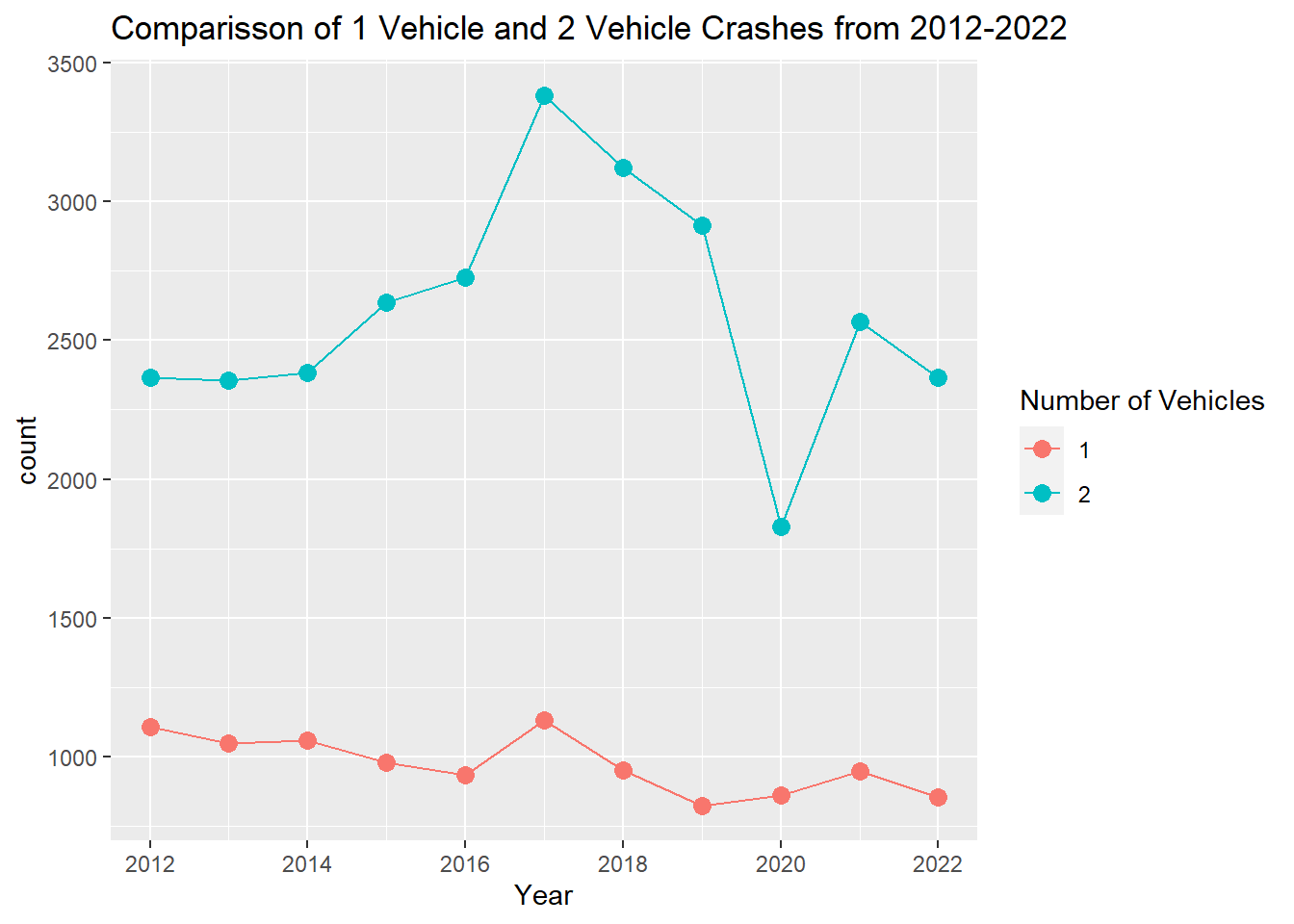
Instances of 2 car crashes have been on an overall trend upwards in Boston, whereas instances of 1 car crashes are decreasing slightly.
Code
vehicles <-mydata%>%select(Year, Number_of_Vehicles)%>%group_by(Year,Number_of_Vehicles)%>%count()vehicles<-pivot_wider(vehicles,names_from=Number_of_Vehicles,values_from = n)vehicles <-mutate_all(vehicles, ~replace_na(.,0))vehicles2<- vehicles%>%pivot_longer(!Year, names_to ="Number_of_Vehicles", values_to ="count")vehicles2 %>%filter(Number_of_Vehicles ==1| Number_of_Vehicles ==2) %>%ggplot(., aes(x=Year, y=`count`, color = Number_of_Vehicles, group=interaction(Number_of_Vehicles))) +geom_point(size=3) +geom_line() +scale_x_continuous(breaks=pretty_breaks()) +labs(title ="Comparisson of 1 Vehicle and 2 Vehicle Crashes from 2012-2022", color ="Number of Vehicles")
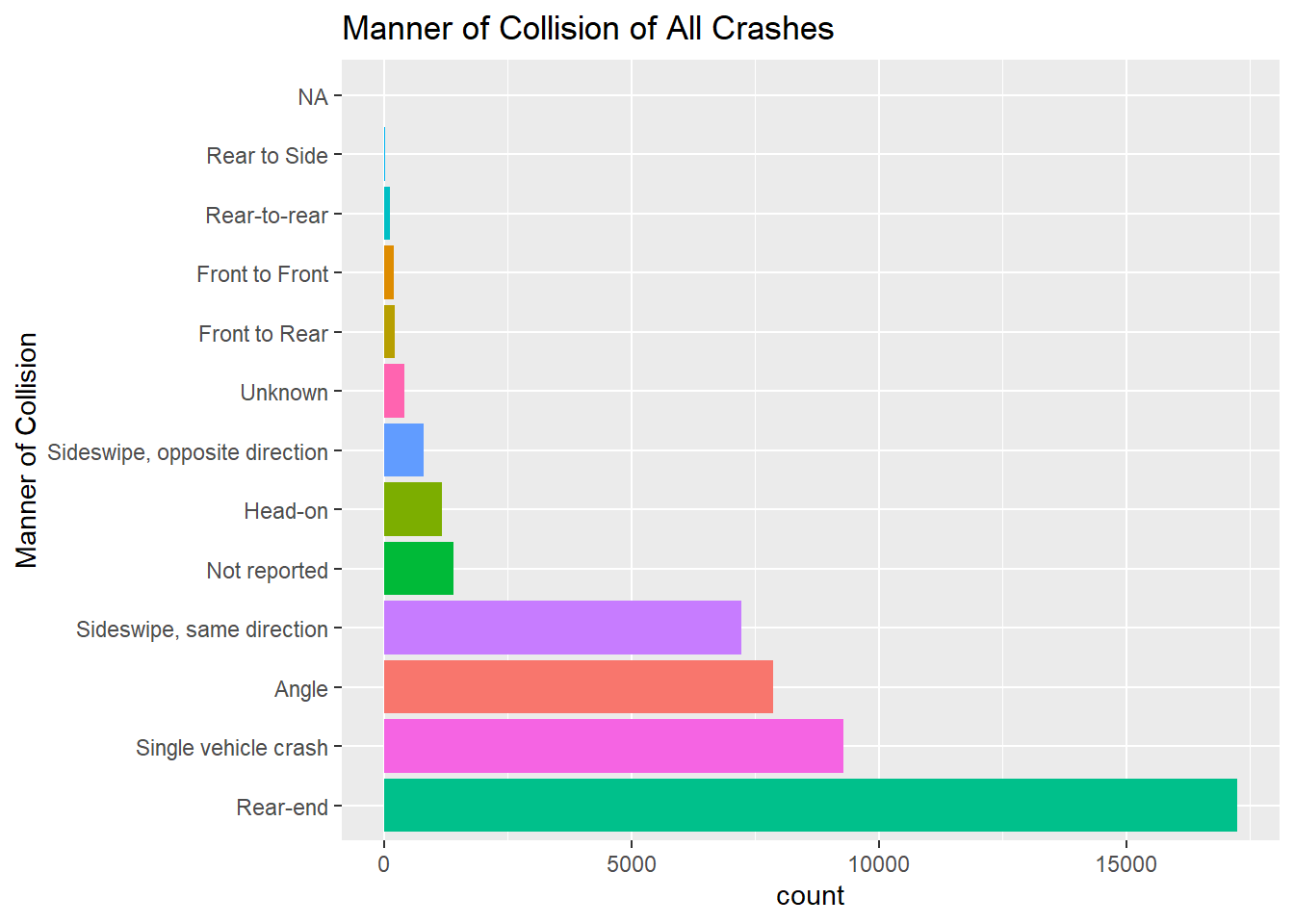
To the surprise of no one (who has driven in the city of Boston), we see that Rear-ends are the manner of collision that occurs most often in Boston.
Following in second, third, and fourth respectively are: Single vehicle crashes, Angle crashes, and Sideswipe, same direction crashes.
Code
mydata %>%ggplot(., aes(x= Manner_of_Collision, stat ="count", fill = Manner_of_Collision)) +geom_bar() +coord_flip() +theme(legend.position ="none") +scale_x_discrete(limits = positions2) +labs(title ="Manner of Collision of All Crashes", x ="Manner of Collision")
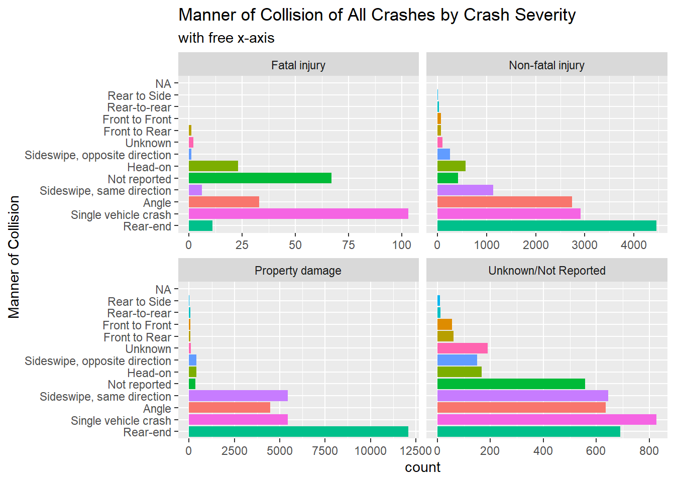
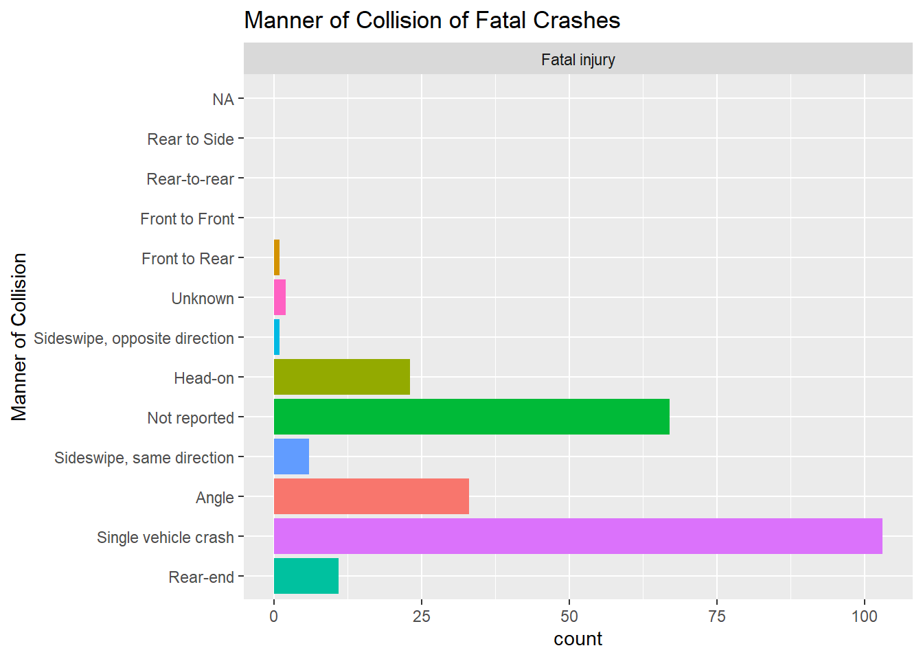
When we subset this data for Crash Severity, we see that fatal injuries occur with the most frequency in single vehicle crashes. The second major difference we see for crashes with fatal injuries is a high proportion of “Not Reported” for manner of collision.
Code
mydata %>%ggplot(aes(x= Manner_of_Collision, stat ="count", fill = Manner_of_Collision)) +geom_bar() +coord_flip() +theme(legend.position ="none") +facet_wrap ( ~ Crash_Severity, scales ="free_x") +scale_x_discrete(limits = positions2) +labs(title ="Manner of Collision of All Crashes by Crash Severity", subtitle ="with free x-axis", x ="Manner of Collision")
Code
mydata %>%filter(Crash_Severity =="Fatal injury") %>%ggplot(aes(x= Manner_of_Collision, stat ="count", fill = Manner_of_Collision)) +geom_bar() +coord_flip() +theme(legend.position ="none") +facet_wrap ( ~ Crash_Severity, scales ="free_x") +scale_x_discrete(limits = positions2) +labs(title ="Manner of Collision of Fatal Crashes", x ="Manner of Collision")
In regards to Crash Severity, the vast majority of crashes in Boston only involve property damage. The lowest proportion, with 0.05% of all crashes, result in fatal injury.
Code
mydataall <- mydata %>%select(Crash_Severity)%>%group_by(Crash_Severity) %>%count()ggplot(mydataall, aes(area= n, fill= Crash_Severity, label =paste0(Crash_Severity, "\n", n))) +geom_treemap() +labs(title ="Crashes in Boston by Severity 2012-2022") +scale_fill_discrete(name ="Crash Severity") +geom_treemap_text(colour ="black",place ="centre") +theme(legend.position ="bottom")
Overall instances of crashes in Boston are changing over time. Two major trends happened: crashes increased from 2012 to 2017, and crashes drastically decreased in 2020. I did not see what I was expecting to see in regards to crashes post-pandemic. As a resident of Boston, I would have assumed accidents had reached their peak in 2022.
Day of the week with the most crashes: Friday
Month with the most crashes: October
Year with the most crashes: 2017
63% of accidents in the city lead to property damage only
What happened in 2017 I still am unclear about, there are certain trends I can parse out in the data but I am left with more questions. Were gas prices really inexpensive in 2017? Were there policies put in place in 2018 to mitigate factors that led to the high rates of crash in 2017?
Next steps
Coordinates! The coordinate data would be fascinating to study. Do sideswipes happen on tight 2 way sidestreets? Do crashes involving pedestrians happen near train stations? Do most rear-ends happen at traffic lights? (Personal anecdote: I got hit by a truck at a red light because the driver was “looking at his gps, and the company truck has bad brakes”)
Number of Vehicles per Crash This was a striking last minute discovery and I’d love to analyze this more. I did not know how to do analysis in R but off screen (on excel) I was able to do some preliminary calculations showing that one car:two car crashes were changing from 1:2 to 1:3 ratio over time and that’s interesting. Does that shed light onto the changing proximity of cars, meaning that more cars, packed in tighter, might mean more cars inevitably involved in a single accident?
Operator Error (utilizing Person Level crash data) MassDot provides person level data involved in each crash. This would have been far too much for me to join person level and crash level data together in this one assignment. However, I would be curious to see what trends have transpired over time. Are more drivers crashing because they are distracted? Are the ages of drivers involved in accidents going up? (I did hear recently that many younger folks are waiting longer to drive, but I have no data to back that up…yet!)
Takeaways
As my first project in R, I bit off quite a lot. I had intended to analyze the coordinates of crashes, however after realizing I needed to understand a fair bit more about the data (and coordinates), I chose to analyze trends over time. This project was hard to start and just as hard to finish, for different reasons. At first I didn’t know how this dataset could yield anything interesting and I thought I’d be bored. Now, as I wrap up the last few words of this report I feel the urge to make “just one more graph!”
References
IMPACT. Data Extract. 2023. https://apps.impact.dot.state.ma.us/cdp/home
INRIX. INRIX 2022 Global Score Card. 2023. http://inrix.com/scorecard/
October Holidays & National Days. National Today. 2023. https://nationaltoday.com/october-holidays/
Source Code
---title: "Final Project: Sue-Ellen Duffy"author: "Sue-Ellen Duffy"description: "Boston Crash Trends 2012-2022"date: "05-20-2023"format: html: df-print: paged toc: true code-fold: true code-copy: true code-tools: true css: "styles.css"categories: - final_project - Sue-Ellen Duffyeditor_options: chunk_output_type: console---```{r}#| label: setup#| warning: false#| message: falselibrary(tidyverse)library(summarytools)library(lubridate)library(ggplot2)library(dplyr)library(hrbrthemes)library(scales)library(sf)library(treemap)library(treemapify)library(timeDate)library(forcats)library(hrbrthemes)library(stringr)library(knitr)library(kableExtra)library(GGally)library(patchwork)knitr::opts_chunk$set(echo =TRUE, warning=FALSE, message=FALSE)```# IntroductionThe dataset was retrieved from the Massachusetts Department of Transportation data extraction service. I requested publicly available crash data for Boston municipality for the specific years of 2012-2022 and received a CSV file. Car crashes are reported to the Registry of Motor Vehicle and from there the Department of Transportation makes data available to the public.This dataset includes 45,980 individual crashes in Boston from 2012-2022 which are represented by each row in the dataset. The dataset includes crash information including date, time, weather and lighting conditions and the severity of each crash. In regards to location, the dataset includes the travel direction of the vehicles, proximity to certain landmarks such as an exit or roadway intersection and the coordinates (latitude and longitude) of the crash point. Post-pandemic car ownership and commuting by car has increased in an astonishing way - not to help the matter, train commutes are slower than ever. This dataset cannot delve deep enough to understand the scope of this transit issue and traffic data is not publicly available. This dataset will at least allow me to analyze city crashes that may yield some understanding about the implications of an increase in car commuting to the city. In a 2022 report by Inrix, Boston ranked 4th on the Global Traffic Scorecard, but not in the good way. ### Questions1. Are crashes in Boston increasing overtime? What type if any are increasing over time? 2. Are there any correlations to time of day, date, or road surface conditions that implicate a higher severity of crash and or more crashes overall?3. How did the pandemic affect Boston crashes?#### Data Description * **Crash Date** - Date occurrence of crash (year, month, and day)* **Crash Time** - Time occurrence of crash (hour, min, and sec)* **Crash Severity** - Indicates the severity of a crash based on the most severe injury to any person based on 3 levels - Fatal injury, Non-fatal injury, Property damage only (no injury) - and either Unknown or Not Reported* **Maximum Injury Severity Reported** - Reported injury if both fatal and non-fatal will be categorized "Fatal injury" as it is the most severe reported injury* **Non_Motorist_Type** - The type of non-motorist * *Crash Hour* - [added for analysis] Time occurrence of crash (hour only) * *Crash Timegroup* - [added for analysis] Time occurrence of crash (defined by time intervals: (Overnight = 2AM-5:59AM; Morning = 6AM-9:59AM; Midday = 10AM-1:59PM; Afternoon = 2PM-5:59PM; Evening = 6PM-9:59PM; Late Night = 10PM-1:59AM)* *Crash Count* - [added for analysis] Number of crash occurrences per day* *Crash Countgroup* - [added for analysis] Number of crash occurrences per day (defined by group intervals: (1-5, 6-10, 11-15, 16-20, 21-25, 26-30, 31-35, 36-40)#### Data Cleaning:```{r}mydataog <-read_csv("Sue-EllenDuffy_FinalProjectData/Crash_Details_2012-2022.csv", skip =2)mydata <- mydataog``````{r}mydataog$Crash_Date <-as.Date(mydataog$Crash_Date, "%d-%b-%Y")mydataog$Year <-year(mydataog$Crash_Date)mydata$Crash_Date <-as.Date(mydata$Crash_Date, "%d-%b-%Y")mydata$Weekday <-wday(mydata$Crash_Date, label =TRUE, abbr =FALSE)mydata$Month <-month(mydata$Crash_Date, label =TRUE, abbr =TRUE)mydata$Year <-year(mydata$Crash_Date)mydata$Day <-day(mydata$Crash_Date)``````{r}mydata<-mydata %>%mutate(Crash_Severity =recode(Crash_Severity, `Property damage only (none injured)`="Property damage",`Unknown`="Unknown/Not Reported", `Not Reported`="Unknown/Not Reported"))``````{r}mydata<-mydata%>%mutate(Crash_Hour=hour(Crash_Time))mydata <- mydata %>%mutate(Crash_Timegroup =case_when(Crash_Hour>=2& Crash_Hour<=5~"Overnight", Crash_Hour>=6& Crash_Hour<=9~"Morning", Crash_Hour>=10& Crash_Hour<=13~"Midday", Crash_Hour>=14& Crash_Hour<=17~"Afternoon", Crash_Hour>=18& Crash_Hour<=21~"Evening", Crash_Hour>=22& Crash_Hour >=23~"Late Night", Crash_Hour>=1& Crash_Hour >=0~"Late Night", Crash_Hour=="0"~"Late Night"))``````{r}mydata<- mydata %>%group_by(Crash_Date) %>%mutate(Crash_Count =n())``````{r}mydata<-mydata%>%mutate(Crash_Countgroup =case_when(Crash_Count>=1& Crash_Count<=5~"1-5", Crash_Count>=6& Crash_Count<=10~"6-10", Crash_Count>=11& Crash_Count<=15~"11-15", Crash_Count>=16& Crash_Count<=20~"16-20", Crash_Count>=21& Crash_Count<=25~"21-25", Crash_Count>=26& Crash_Count<=30~"26-30", Crash_Count>=31& Crash_Count<=35~"31-35", Crash_Count>=36& Crash_Count<=40~"36-40"))``````{r}positionroad <-c("Wet", "Snow", "Water standing, moving)", "Slush", "Sand, mud, dirt, oil, gravel", "NA", "Unknown", "Not reported", "Ice", "Dry")positions <-c("Overnight", "Morning", "Midday", "Afternoon", "Evening", "Late Night")positions2 <-c("Rear-end", "Single vehicle crash", "Angle", "Sideswipe, same direction", "Not reported", "Head-on", "Sideswipe, opposite direction", "Unknown", "Front to Rear", "Front to Front", "Rear-to-rear", "Rear to Side", "NA")position_Countgroup <-c("1-5", "6-10", "11-15", "16-20", "21-25", "26-30", "31-35", "36-40")```#### Handling Unknown, Not Reported, NA or Missing data**Unknown/Not Reported Data:** There were 45,980 crashes reported from 2012 to 2022. Of those crashes 4,002 (8.7%) were reported with a Crash Severity of "Unknown" or "Not Reported" the majority are reported as resulting in property damage only with no injuries reported. Ranking second is non-fatal injuries, and finally a small portion are rated as fatal injuries. + For the purpose of this report, and for the category of "Crash Severity" only, I have combined these into "Unknown/Not Reported". **Why are some crashes reported as Unknown or Not Reported? Possibilities include:** + internal clerical errors + reports must be completed within 5 days of crash (leading to rushed answers) + decision fatigue from having to fill out the report alone post accident + data missing due to personal choice in managing insurance claims**Unknown/Not Reported Over Time:** The category "Unknown" was used more so in later years, with a peak in 2021. Whereas "Not Reported" had peaks in 2012 and 2017 and very low numbers in 2020-2022.```{r}pUnknown <- mydataog %>%filter(Crash_Severity =="Unknown") %>%ggplot(., aes(x=Year)) +geom_bar() +facet_wrap( ~ Crash_Severity, ) +theme(legend.position ="none") +scale_x_continuous(breaks=pretty_breaks()) +coord_cartesian(ylim =c(0, 700))pNotReported <- mydataog %>%filter(Crash_Severity =="Not Reported") %>%ggplot(., aes(x=Year)) +geom_bar() +facet_wrap( ~ Crash_Severity, ) +theme(legend.position ="none") +scale_x_continuous(breaks=pretty_breaks())ppUN <- (pUnknown + pNotReported)ppUN +plot_annotation(title ="Reports of 'Unknown' and 'Not Reported' for category Crash Severity")```**Unknown/Not Reported Data Inconsistencies:**Crashes that were reported under Crash Severity as being "Unknown" or "Not Reported" had 50 inconsistently reported injuries in another column of the data. All 50 reporting inconsistencies occurred between May 2018 and October 2019: * Crash Severity "Not Reported" has 42 reports of maximum injury reports across 6 categories that suggest a possible injury. * Crash Severity "Unknown" has 7 reports of non-fatal injury as either "Non-incapacitating" or "Possible" and 1 report of "No apparent injury". ```{r}mydataog <- mydataog %>%mutate(Crash_Severity =recode(Crash_Severity, `Property damage only (none injured)`="Property damage"))mydatainconsistencies <- mydataog %>%filter(between(Crash_Date, as.Date('2018-05-01'), as.Date('2019-10-31'))) ```**Missing data/NAs and outliers:** Road Surface Condition has an NA count of n=368. For the purpose of this report I am considering this sort of NA to be comparable with "Not Reported" or "Unknown" and leave the data in the dataset as I am only looking at a few indicators of Road Surface Condition and not analyzing it in depth. Manner of Collision also has an NA count of n=5. I will leave that data alone as well.# Overview of Crash Data in Boston 2012-2022```{r}ggplot(mydata, aes(Crash_Date, stat="count")) +geom_bar() +labs(x="Crash Date", y="Crashes per Day", title ="Crash Data from 2012-2022, Boston")```::: panel-tabset## DailyBoston averaged 13 crashes per day (from 2012-2022). ```{r}#Crash Count per Daymydatacountsall <- mydata %>%group_by(City_Town_Name) %>%summarize("min"=min(Crash_Count, na.rm =TRUE),"max"=max(Crash_Count, na.rm =TRUE),"mean"=mean(Crash_Count, na.rm =TRUE), "median"=median(Crash_Count, na.rm =TRUE),"standard deviation"=sd(Crash_Count, na.rm =TRUE)) %>%arrange(City_Town_Name)mydatacountsall%>%kbl() %>%kable_classic()```By viewing daily crash counts in intervals of 5 we can see that on most days there are 11-15 crashes in Boston, with some days having 6-10 or 16-20 crashes. Very few days have 5 or less crashes.```{r}ggplot(mydata, aes(Crash_Countgroup, stat="count")) +geom_bar() +scale_x_discrete(limit =position_Countgroup) +labs(title ="Crashes by Daily Crash Count Groups", x ="Count Groups")```The following graph shows the density of crashes with crash counts per day. As opposed to the bargraph charting all crashes by total counts in the Overview, this graph lets us see outliers not only in the top portion of the graph with the most counts, but also in the lowest counts. We can now see the pockets of time when there were, for instance, more than 6 crashes per day everyday, like in 2017, or the time when in 2020 there were many instances of having only a 1-3 crashes per day.```{r}ggplot(mydata, aes(Crash_Date, y=Crash_Count, group = Crash_Severity)) +geom_point() +geom_jitter() +labs(title ="All Crashes by Date", y ="Crash counts per day", x ="Date")```## Day of the WeekBoston saw the most crashes on Fridays (2012-2022).```{r}mydata %>%ggplot(aes(Weekday, fill = Weekday)) +geom_bar( stat ="count") +theme(axis.text.x =element_text(angle =90)) +theme(legend.position ="none") +labs(title ="Days of the Week & Crash Count", x ="")```When subsetted for Crash Severity, however Boston sees the most fatal accidents on Wednesday and Saturday. (The following graph shows Crash Severity: Fatal injury, Non-fatal injury, and Property damage. It does not include Unknown/Not Reported)```{r}mydata %>%filter(Crash_Severity !="Unknown/Not Reported") %>%ggplot(aes(Weekday, fill = Weekday)) +geom_bar( stat ="count") +facet_wrap ( ~ Crash_Severity, scales ="free_y") +theme(axis.text.x =element_text(angle =90)) +theme(legend.position ="none") +labs(title ="Days of the Week & Crash Severity", subtitle ="with free Y-axis", x ="") ```## MonthOctober is the month with the most crashes and the highest average crash rate in Boston (2012-2022), averaging 15 crashes per day. Buckle up, this tab has a longer analysis section.```{r}#Crash Count per Day by Monthmydatamonthsum <- mydata %>%group_by(Month) %>%summarize("min"=min(Crash_Count, na.rm =TRUE),"max"=max(Crash_Count, na.rm =TRUE),"mean"=mean(Crash_Count, na.rm =TRUE), "median"=median(Crash_Count, na.rm =TRUE),"standard_deviation"=sd(Crash_Count, na.rm =TRUE))%>%arrange(Month)mydatamonthsum %>%kbl(caption ="Crash Statistic by Month") %>%kable_classic() %>%row_spec(10, bold = T, color ="black", background ="orange") ``````{r}ggplot(mydata, aes(Month, stat="count")) +geom_bar() +labs(title ="All Crashes by Month")```### What could we learn about October? + Do road conditions have something to do with the increase in accidents? + Are there different types of accidents in October? + Is it all happening around Halloween? #### Road Surface ConditionsWhen we subset the data for October by road surface condition we see that "dry" is the predominant condition, however we see "Wet" with a large portion of data as well. ```{r}wet1 <- mydata %>%filter(Month =="Oct") %>%ggplot(., aes(Road_Surface_Condition, stat ="count", fill = (Road_Surface_Condition =="Wet"))) +geom_bar() +coord_flip() +labs(x ="Road Surface", y ="", title =str_wrap("October Crashes by Road Surface Condition", width =25)) +scale_x_discrete(labels =function(x) str_wrap(x, width =5))+theme(legend.position ="none") +scale_fill_manual(values=c( "#999999", "#0000FF"))wet2 <- mydata %>%filter(Road_Surface_Condition =="Wet") %>%ggplot(., aes(Road_Surface_Condition, stat ="count", fill = Month)) +geom_bar() +facet_wrap( ~ Month,) +labs(x ="", title =str_wrap("All Crashes with Road Surface Condition 'Wet' by Month", width =25)) +theme(legend.position ="none") +scale_fill_manual(values=c("#B7DFF6", "#B7DFF6", "#B7DFF6", "#B7DFF6", "#B7DFF6", "#B7DFF6", "#B7DFF6", "#B7DFF6", "#B7DFF6", "#0000FF", "#B7DFF6", "#B7DFF6"))wet1 + wet2```While October has the most crashes with "Wet" road surface conditions reported, October also has the most crashes overall. In order to understand whether this road surface condition "Wet" was a factor in making October the month with the highest crash rating, I looked at the percentages of crashes in each month that occurred under "Wet" road surface conditions. October and December both have 25% of crashes (per their respective months) with "Wet" road surface conditions reported.```{r}mydata %>%ggplot(., aes(Month, stat ="count", fill = (Road_Surface_Condition =="Wet"))) +geom_bar(position ="fill") +labs(title ="Crashes with Road Surface Condition 'Wet' by Month", y ="percent", x ="Month", fill ="Wet") +scale_fill_manual(values=c("#999999", "#B7DFF6", "#999999"))``````{r}road<-mydata%>%select(Month, Road_Surface_Condition)%>%group_by(Month,Road_Surface_Condition)%>%count()road<-pivot_wider(road,names_from=Road_Surface_Condition,values_from = n)road <-mutate_all(road, ~replace_na(.,0))road <- road %>%mutate(total =sum(c_across(Dry:Wet))) %>%ungroup() %>%mutate(across(Dry:"NA", ~ ./ total)) %>%mutate(across(Dry:"NA", ~ .*100))road %>%kbl(digits =1, caption ="Road Conditions of Crashes (2012-2022) by Month") %>%kable_classic() %>%column_spec(11, bold = T) %>%row_spec(c(10, 12), color ="black", background ="#B7DFF6") ```#### Non-Motorist InvolvementOctober is the month with the most instances of Non-motorist type involvement in crashes with 253 reports.```{r}nm<-mydata%>%select(Month, Non_Motorist_Type)%>%group_by(Month,Non_Motorist_Type)%>%count()nm<-pivot_wider(nm,names_from=Non_Motorist_Type,values_from = n)nm <-mutate_all(nm, ~replace_na(.,0))nm <- nm %>%select(., -"NA")nm <-nm %>%mutate(total =sum(c_across("P1: Pedestrian":"P2: Cyclist / P3: Other / P4: Other"))) %>%ungroup() nm <- nm %>%mutate(across("P1: Pedestrian":"P2: Cyclist / P3: Other / P4: Other" , ~ ./ total)) %>%mutate(across("P1: Pedestrian":"P2: Cyclist / P3: Other / P4: Other", ~ .*100))#total instances of crashes with Non-Motorists reported by Monthggplot(nm, aes(x=Month, y = total)) +geom_point() +labs(title ="Crashes Involving Non-Motorists")```However proportional to the total number of crashes per Month, we see that July and September have the highest % of crashes involving non-motorist types.```{r}mydata %>%ggplot(., aes(Month, stat ="count", fill = (Non_Motorist_Type !="NA"))) +geom_bar(position ="fill") +labs(title ="Percent Crashes per Month Involving Non-Motorists", y ="percent", fill ="Non-Motorist Involved")```#### Crash SeverityLet's look at how each crash severity rating factors into this month analysis.We can now see that the month with the highest Fatal injury is reported in July, with dips in spring, winter, and October while Non-fatal injuries and Property damage peak in October. The peak for Unknown/Not Reported crashes is in May and June.```{r}ggplot(mydata, aes(Month, stat="count", fill = Crash_Severity)) +geom_bar() +facet_wrap( ~ Crash_Severity, scales ="free_y") +labs(title ="Crash Severity by Month", subtitle ="with free y-axis") +theme(legend.position ="none")```#### Dates within OctoberI can't call Halloween out on this one.October 4th has the most counts of crashes in the month, which happens to be National Taco Day and World Animal Day. ```{r}mydata %>%filter(Month =="Oct") %>%ggplot(., aes(x =Day, stat ="count", fill = (Day =="31"))) +geom_bar() +scale_fill_manual(values=c("#999999", "orange"))+labs(title ="Crash Counts by Day in October", x ="Days in October", fill ="Halloween")```## Year2017 was the year with the most crashes in Boston (2012-2022).```{r}#Crash Count per Day by Yearmydatasum <- mydata %>%group_by(Year) %>%summarize("min"=min(Crash_Count, na.rm =TRUE),"max"=max(Crash_Count, na.rm =TRUE),"mean"=mean(Crash_Count, na.rm =TRUE), "median"=median(Crash_Count, na.rm =TRUE),"standard deviation"=sd(Crash_Count, na.rm =TRUE)) %>%arrange(Year)mydatasum %>%kbl(caption ="Crash Statistic by Year") %>%kable_classic() %>%row_spec(6, bold = T) ```The data shows 2017 as a peak with a sharp drop off in 2020 (due to the pandemic and reduced traffic flow) then a climb back up in 2021 almost matching crash reports from 2019. Of course this data shows that post-pandemic rates of car crashes have gone back up, but it is not as high as crashes in 2017.```{r}ggplot(mydata, aes(year(Crash_Date))) +geom_histogram(binwidth = .50) +scale_x_continuous(breaks=pretty_breaks()) +labs(title ="All Crashes by Year", x ="Year",)```### What happened in 2017 and were these crashes somehow different from crashes in other years?#### Road Surface Conditions2017 had the most incidents of crash where "Ice" was the indicated road surface condition. Not the most significant data point considering its low n(79) but interesting none the less.```{r}datayear <- mydatadatayear =table(datayear$Year, datayear$Road_Surface_Condition) datayear %>%kbl(caption ="Road Conditions of Crashes (2012-2022) by Year" ) %>%kable_classic() %>%column_spec(3, bold = T) %>%row_spec(6, color ="black", background ="#B7DFF6")```#### Number of Vehicles Involved 2017 had the most **2 car** accidents and had 1 instance each of a **12 car** and **18 car** crash. Both of these high number crashes were in fact Ice related. - *While a crash may involve multiple cars, the counts recorded throughout the data and this analysis are on individual crashes (regardless of how many cars are involved in the crash)*```{r}#Year and Number of Vehiclesdatayearvehicles <- mydatadatayearvehicles =table(datayearvehicles$Year, datayearvehicles$Number_of_Vehicles) datayearvehicles %>%kbl(caption ="Number of Vehicles Involved in Crashes (2012-2022) by Year" ) %>%kable_classic() %>%column_spec(3:4, bold = T) %>%row_spec(6, color ="black", background ="#B7DFF6")```#### Non-Motorists Involved2017 is the year with the most crashes involving Non-Motorists with 378 crashes.```{r}#Year and Non-motorist Typenmy<-mydata%>%select(Year, Non_Motorist_Type)%>%group_by(Year,Non_Motorist_Type)%>%count()nmy<-pivot_wider(nmy,names_from=Non_Motorist_Type,values_from = n)nmy <-mutate_all(nmy, ~replace_na(.,0))nmy <- nmy %>%select(., -"NA")nmy <-nmy %>%mutate(total =sum(c_across("P1: Cyclist":"P9: Pedestrian"))) %>%ungroup() nmy <- nmy %>%mutate(across("P1: Cyclist":"P9: Pedestrian" , ~ ./ total)) %>%mutate(across("P1: Cyclist":"P9: Pedestrian", ~ .*100))ggplot(nmy, aes(x=Year, y = total)) +geom_point() +scale_x_continuous(breaks=pretty_breaks()) +labs(title ="Crashes Involving Non-Motorist by Year")```However, again, while it has the most instances of Non-motorist involvement, 2017 has just about the same percent of crashes as 2012 and 2013, with around 7% of all crashes in each of those years involving non-motorists```{r}mydata %>%ggplot(., aes(Year, stat ="count", fill = (Non_Motorist_Type !="NA"))) +geom_bar(position ="fill") +scale_x_continuous(breaks=pretty_breaks()) +labs(title ="Percent Crashes per Year Involving Non-Motorists", y ="percent", fill ="Non-Motorist Involved")```## Time of DayMost crashes occur in the afternoon, between 3pm and 5pm, in Boston (2012-2022).```{r}ggplot(mydata, aes(Crash_Hour)) +geom_histogram(stat="count") +labs(title ="Crashes by Hour of Crash", x ="Hour of Crash")```While Non-fatal, Property damage, Unknown/Not Reported all follow the same pattern of peaks in the afternoon, crashes resulting in Fatal injury peak at late night.*Time occurrence of crash (defined by time intervals: (Overnight = 2AM-5:59AM; Morning = 6AM-9:59AM; Midday = 10AM-1:59PM; Afternoon = 2PM-5:59PM; Evening = 6PM-9:59PM; Late Night = 10PM-1:59AM)*```{r}tgroup <-ggplot(mydata, aes(Crash_Timegroup, stat="count", fill = Crash_Severity)) +geom_bar() +scale_x_discrete(limits = positions) +labs(title ="Crashes by Time Group", x ="Time Group", fill ="Crash Severity") +theme(legend.position ="none")csgroup <-ggplot(mydata, aes(Crash_Timegroup, stat="count", fill = Crash_Severity)) +geom_bar() +facet_wrap ( ~ Crash_Severity, scales ="free_y") +scale_x_discrete(limits = positions) +theme(legend.position ="none") +labs(x ="Time Group", subtitle ="with free y-axis", title =str_wrap("Time Group and Crash Severity", width =40)) +theme(axis.text.x =element_text(angle =90))tgroup + csgroup```## Number of Vehicles per CrashInstances of 2 car crashes have been on an overall trend upwards in Boston, whereas instances of 1 car crashes are decreasing slightly.```{r}vehicles <-mydata%>%select(Year, Number_of_Vehicles)%>%group_by(Year,Number_of_Vehicles)%>%count()vehicles<-pivot_wider(vehicles,names_from=Number_of_Vehicles,values_from = n)vehicles <-mutate_all(vehicles, ~replace_na(.,0))vehicles2<- vehicles%>%pivot_longer(!Year, names_to ="Number_of_Vehicles", values_to ="count")vehicles2 %>%filter(Number_of_Vehicles ==1| Number_of_Vehicles ==2) %>%ggplot(., aes(x=Year, y=`count`, color = Number_of_Vehicles, group=interaction(Number_of_Vehicles))) +geom_point(size=3) +geom_line() +scale_x_continuous(breaks=pretty_breaks()) +labs(title ="Comparisson of 1 Vehicle and 2 Vehicle Crashes from 2012-2022", color ="Number of Vehicles")```## Manner of CollisionTo the surprise of no one (who has driven in the city of Boston), we see that Rear-ends are the manner of collision that occurs most often in Boston. Following in second, third, and fourth respectively are: Single vehicle crashes, Angle crashes, and Sideswipe, same direction crashes.```{r}mydata %>%ggplot(., aes(x= Manner_of_Collision, stat ="count", fill = Manner_of_Collision)) +geom_bar() +coord_flip() +theme(legend.position ="none") +scale_x_discrete(limits = positions2) +labs(title ="Manner of Collision of All Crashes", x ="Manner of Collision")```When we subset this data for Crash Severity, we see that fatal injuries occur with the most frequency in single vehicle crashes. The second major difference we see for crashes with fatal injuries is a high proportion of "Not Reported" for manner of collision. ```{r}mydata %>%ggplot(aes(x= Manner_of_Collision, stat ="count", fill = Manner_of_Collision)) +geom_bar() +coord_flip() +theme(legend.position ="none") +facet_wrap ( ~ Crash_Severity, scales ="free_x") +scale_x_discrete(limits = positions2) +labs(title ="Manner of Collision of All Crashes by Crash Severity", subtitle ="with free x-axis", x ="Manner of Collision")mydata %>%filter(Crash_Severity =="Fatal injury") %>%ggplot(aes(x= Manner_of_Collision, stat ="count", fill = Manner_of_Collision)) +geom_bar() +coord_flip() +theme(legend.position ="none") +facet_wrap ( ~ Crash_Severity, scales ="free_x") +scale_x_discrete(limits = positions2) +labs(title ="Manner of Collision of Fatal Crashes", x ="Manner of Collision")```## Crash SeverityIn regards to Crash Severity, the vast majority of crashes in Boston only involve property damage. The lowest proportion, with 0.05% of all crashes, result in fatal injury.```{r}mydataall <- mydata %>%select(Crash_Severity)%>%group_by(Crash_Severity) %>%count()ggplot(mydataall, aes(area= n, fill= Crash_Severity, label =paste0(Crash_Severity, "\n", n))) +geom_treemap() +labs(title ="Crashes in Boston by Severity 2012-2022") +scale_fill_discrete(name ="Crash Severity") +geom_treemap_text(colour ="black",place ="centre") +theme(legend.position ="bottom") ``````{r}tabseverities <-table(mydata$City_Town_Name, mydata$Crash_Severity)kable(tabseverities)```:::## Final Conclusion and TakeawaysOverall instances of crashes in Boston are changing over time. Two major trends happened: crashes increased from 2012 to 2017, and crashes drastically decreased in 2020. I did not see what I was expecting to see in regards to crashes post-pandemic. As a resident of Boston, I would have assumed accidents had reached their peak in 2022. + Day of the week with the most crashes: Friday+ Month with the most crashes: October+ Year with the most crashes: 2017+ 63% of accidents in the city lead to property damage onlyWhat happened in 2017 I still am unclear about, there are certain trends I can parse out in the data but I am left with more questions. Were gas prices really inexpensive in 2017? Were there policies put in place in 2018 to mitigate factors that led to the high rates of crash in 2017? ### Next steps**Coordinates!**The coordinate data would be fascinating to study. Do sideswipes happen on tight 2 way sidestreets? Do crashes involving pedestrians happen near train stations? Do most rear-ends happen at traffic lights? (Personal anecdote: I got hit by a truck at a red light because the driver was "looking at his gps, and the company truck has bad brakes")**Number of Vehicles per Crash**This was a striking last minute discovery and I'd love to analyze this more. I did not know how to do analysis in R but off screen (on excel) I was able to do some preliminary calculations showing that one car:two car crashes were changing from 1:2 to 1:3 ratio over time and that's interesting. Does that shed light onto the changing proximity of cars, meaning that more cars, packed in tighter, might mean more cars inevitably involved in a single accident?**Operator Error (utilizing Person Level crash data)**MassDot provides person level data involved in each crash. This would have been far too much for me to join person level and crash level data together in this one assignment. However, I would be curious to see what trends have transpired over time. Are more drivers crashing because they are distracted? Are the ages of drivers involved in accidents going up? (I did hear recently that many younger folks are waiting longer to drive, but I have no data to back that up...yet!)### TakeawaysAs my first project in R, I bit off quite a lot. I had intended to analyze the coordinates of crashes, however after realizing I needed to understand a fair bit more about the data (and coordinates), I chose to analyze trends over time.This project was hard to start and just as hard to finish, for different reasons. At first I didn't know how this dataset could yield anything interesting and I thought I'd be bored. Now, as I wrap up the last few words of this report I feel the urge to make "just one more graph!"### References+ IMPACT. Data Extract. 2023. https://apps.impact.dot.state.ma.us/cdp/home+ INRIX. INRIX 2022 Global Score Card. 2023. http://inrix.com/scorecard/+ October Holidays & National Days. National Today. 2023. https://nationaltoday.com/october-holidays/