library(tidyverse)
library(summarytools)
library(lubridate)
library(ggplot2)
library(dplyr)
library(hrbrthemes)
library(scales)
library(sf)
library(plotly)
library(timeDate)
library(forcats)
library(hrbrthemes)
library(stringr)
knitr::opts_chunk$set(echo = TRUE, warning=FALSE, message=FALSE)Final Project Assignment#2: Sue-Ellen Duffy
final_Project_assignment_2
final_project_data_visualization
Exploratory Analysis and Visualization
Part 1. Introduction
- Data Introduction
The dataset was retrieved from the Massachusetts Department of Transportation data extraction service. I requested publicly available crash data for Boston municipality for the specific years of 2012-2022 and received a CSV file.
This dataset includes 45,980 individual crashes in Boston from 2012-2022 which are represented by each row in the dataset. The dataset includes crash information including date, time, weather and lighting conditions and the severity of each crash. In regards to location, the dataset includes the travel direction of the vehicles, proximity to certain landmarks such as an exit or roadway intersection and the coordinates (latitude and longitude) of the crash point. There are insert number of different data points per crash with some NAs or Unreported or Missing information.
Post-pandemic car ownership and commuting by car has increased in an astonishing way - not to help the matter, train commutes are slower than ever. This dataset cannot delve deep enough to understand the scope of this transit issue and traffic data is not publicly available. This dataset will at least allow me to analyze city crashes that may yield some understanding about the implications of an increase in car commuting to the city. Insert some data from Inrix Potentially mention Vision Zero Boston
Questions
Are crashes in Boston increasing overtime? What type if any are increasing over time?
Are there any correlations to time of day, date, or weather conditions that implicate a higher severity of crash and or a higher prevalence/count of crash.
How did the pandemic affect Boston crashes?
Part 2. Describe the data set
mydataog <- read_csv("Sue-EllenDuffy_FinalProjectData/Crash_Details_2012-2022.csv",
    skip = 2)
mydata <- mydataogmydata$Crash_Date <- as.Date(mydata$Crash_Date, "%d-%b-%Y")
mydata$Weekday <-wday(mydata$Crash_Date, label = TRUE, abbr = FALSE)
mydata$Month <- month(mydata$Crash_Date, label = TRUE, abbr = TRUE)
mydata$Year <- year(mydata$Crash_Date)mydata<-mydata %>%
mutate(Crash_Severity = recode(Crash_Severity, `Property damage only (none injured)` = "Property damage",
`Unknown` = "Unknown/Not Reported", `Not Reported` = "Unknown/Not Reported"))mydata<-mydata%>%
mutate(Crash_Hour=hour(Crash_Time))
mydata <- mydata %>%
mutate(Crash_Timegroup = case_when(Crash_Hour>=6 & Crash_Hour<=9 ~ "Morning", Crash_Hour>=10 & Crash_Hour<= 13 ~ "Midday", Crash_Hour>=14 & Crash_Hour<=17 ~ "Afternoon", Crash_Hour>=18 & Crash_Hour<=21 ~ "Evening", Crash_Hour>= 22 & Crash_Hour >=23 ~ "Late Night", Crash_Hour>= 1 & Crash_Hour >=0 ~ "Late Night", Crash_Hour== "0" ~ "Late Night",Crash_Hour>=2 & Crash_Hour<=5 ~ "Overnight"))mydata<- mydata %>%
group_by(Crash_Date) %>%
mutate(Crash_Count = n())mydata<-mydata%>%
mutate(Crash_Countgroup =
case_when(Crash_Count>=1 & Crash_Count<= 5 ~ "1-5",
Crash_Count>=6 & Crash_Count<=10 ~ "6-10",
Crash_Count>=11 & Crash_Count<=15 ~ "11-15",
Crash_Count>= 16 & Crash_Count<=20 ~ "16-20",
Crash_Count>=21 & Crash_Count<=30 ~ "21-30",
Crash_Count>=31 & Crash_Count<=50 ~ "31-37"))dim(mydata)[1] 45980 32head(mydata)Columns/Data Description - from original data
Crash_Date - Date occurrence of crash (year, month, and day)
Crash_Time - Time occurrence of crash (hour, min, and sec)
Crash_Severity - Indicates the severity of a crash based on the most severe injury to any person based on 3 levels - Fatal injury,
Non-fatal injury, Property damage only (no injury) - and either Unknown or Not Reported
Maximum_Injury_Severity_Reported - Reported injury if both fatal and non-fatal will be categorized “Fatal injury” as it is the most severe reported injury
Number_of_Vehicles - Number of vehicles involved in crash occurrence
Total_Nonfatal_Injuries -
Total_Fatal_Injuries -
Weather_Condition - The prevailing and secondary (if applicable) atmospheric conditions at the time of crash
Non_Motorist_Type - The type of non-motorist
Columns/Data Description - added for analysis
Crash_Hour - Time occurrence of crash (hour only)
Crash_Timegroup - Time occurrence of crash (time intervals - fill this in)
Crash_Count - Number of crash occurrences per day
Crash_Countgroup - Number of crash occurrences per day (defined by group intervals - fill this in)
Date and Time Tidying
Sanity Check - Any Crashes reported more than once? No. Duplicate was run and the row counts remained the same. > mydata[!duplicated(mydata$Crash_Number), ] # A tibble: 45,980 × 28 >
Part 3. Visualization
Crash Data by Severity
There were 45,980 reported from 2012 to 2022. Of those crashes the majority are reported as resulting in property damage only with no injuries reported. Ranking second is non-fatal injuries, and finally a small portion are rated as fatal injuries. 4,002 crashes, while reported to MassDot are missing report data on crash severity and are reported as “Unknown” or “Not Reported. For the purpose of this report, I have combined this category into”Unknown/Not Reported”. These “Unknown/Not Reported” crashes make up 8.7% of the crash data but we do not know the crash severity and therefore cannot use this data during certain analysis. In the following data I will note on each graph if I have removed these missing data from analysis.
tabseverities <- table(mydata$City_Town_Name, mydata$Crash_Severity)
tabseverities
         Fatal injury Non-fatal injury Property damage Unknown/Not Reported
BOSTON 248 12804 28926 4002ggplot(mydata, aes(x=Crash_Severity, fill = Crash_Severity)) + geom_histogram(stat = "count") 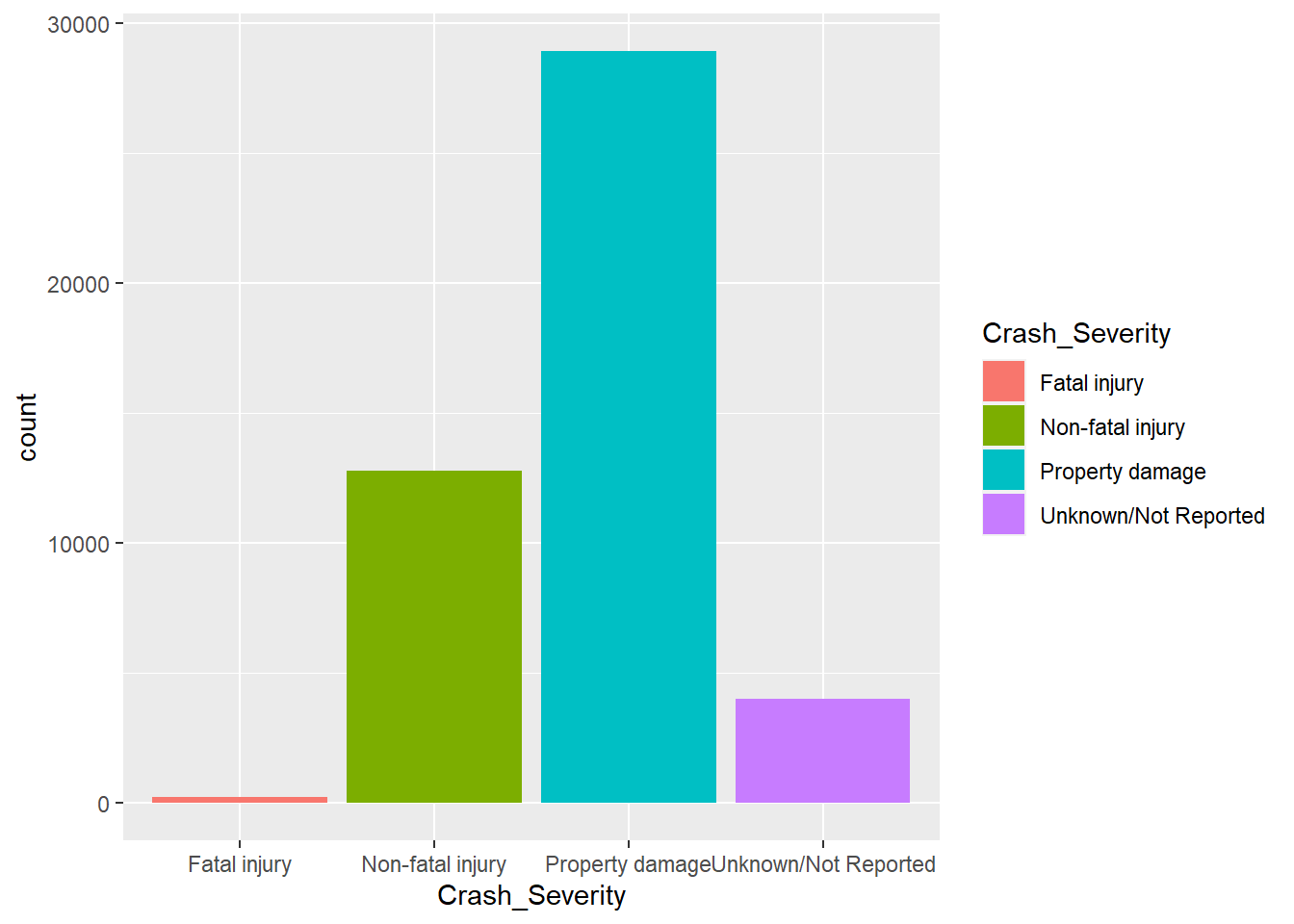
Crash Data by Date/Time
Overall Data
allplot<- ggplot(mydata, aes(Crash_Date, stat="count")) + geom_bar()
ggplotly(allplot)ggplot(mydata, aes(Crash_Date, y=Crash_Count, group = Crash_Severity)) + geom_point()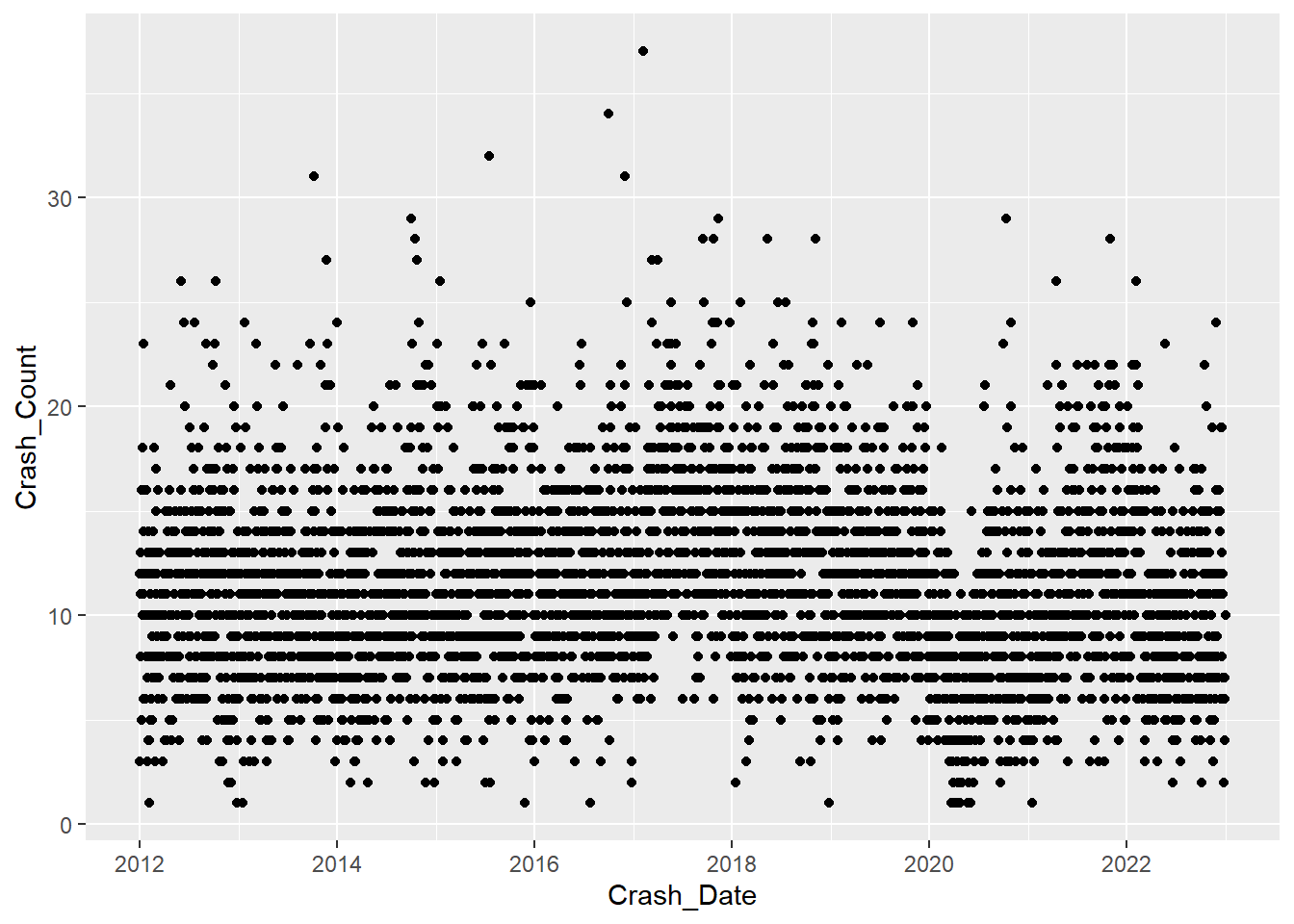
Crash Data by Day
Boston Averages 13 crashes per day (from 2012-2022).
#Crash Count per Day
mydatacountsall <- mydata %>%
  group_by(City_Town_Name) %>%
  summarize("min" = min(Crash_Count, na.rm = TRUE),
            "max" = max(Crash_Count, na.rm = TRUE),
            "mean" = mean(Crash_Count, na.rm = TRUE),
            "median" = median(Crash_Count, na.rm = TRUE),
            "standard_deviation" = sd(Crash_Count, na.rm = TRUE)) %>%
  arrange(City_Town_Name)
print(mydatacountsall)
# A tibble: 1 × 6
City_Town_Name min max mean median standard_deviation
<chr> <int> <int> <dbl> <dbl> <dbl>
1 BOSTON 1 37 13.2 13 4.68position_Countgroup <- c("1-5", "6-10", "11-15", "16-20", "21-30", "31-37")
ggplot(mydata, aes(Crash_Countgroup, stat="count")) + geom_bar() + scale_x_discrete(limit =position_Countgroup)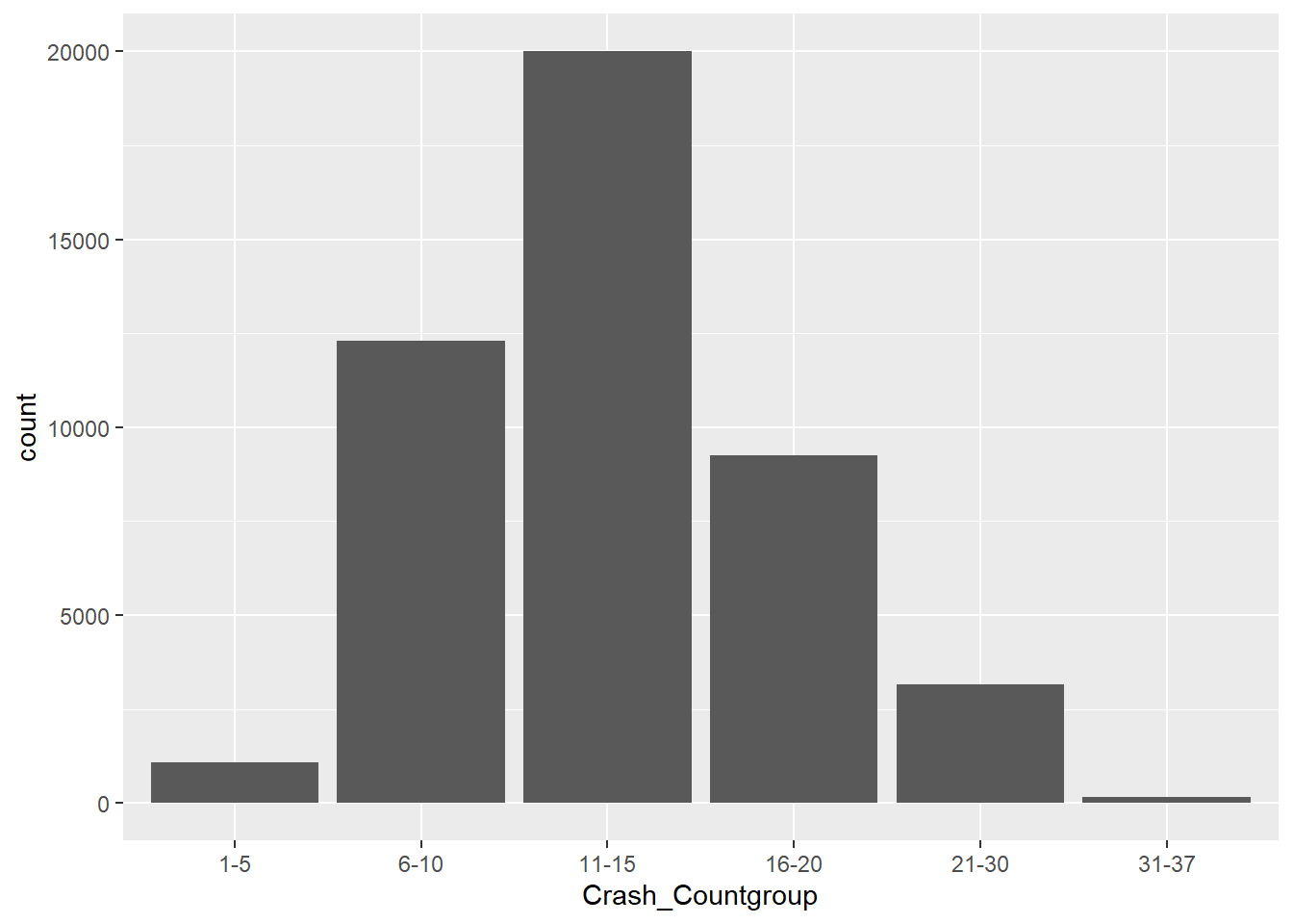
Crash Data by Day of the Week
Overall, Boston sees the most crashes on Friday.
mydata %>%
ggplot(aes(Weekday, fill = Weekday)) +
  geom_bar( stat = "count") + theme(axis.text.x = element_text(angle = 90)) + theme(legend.position = "none")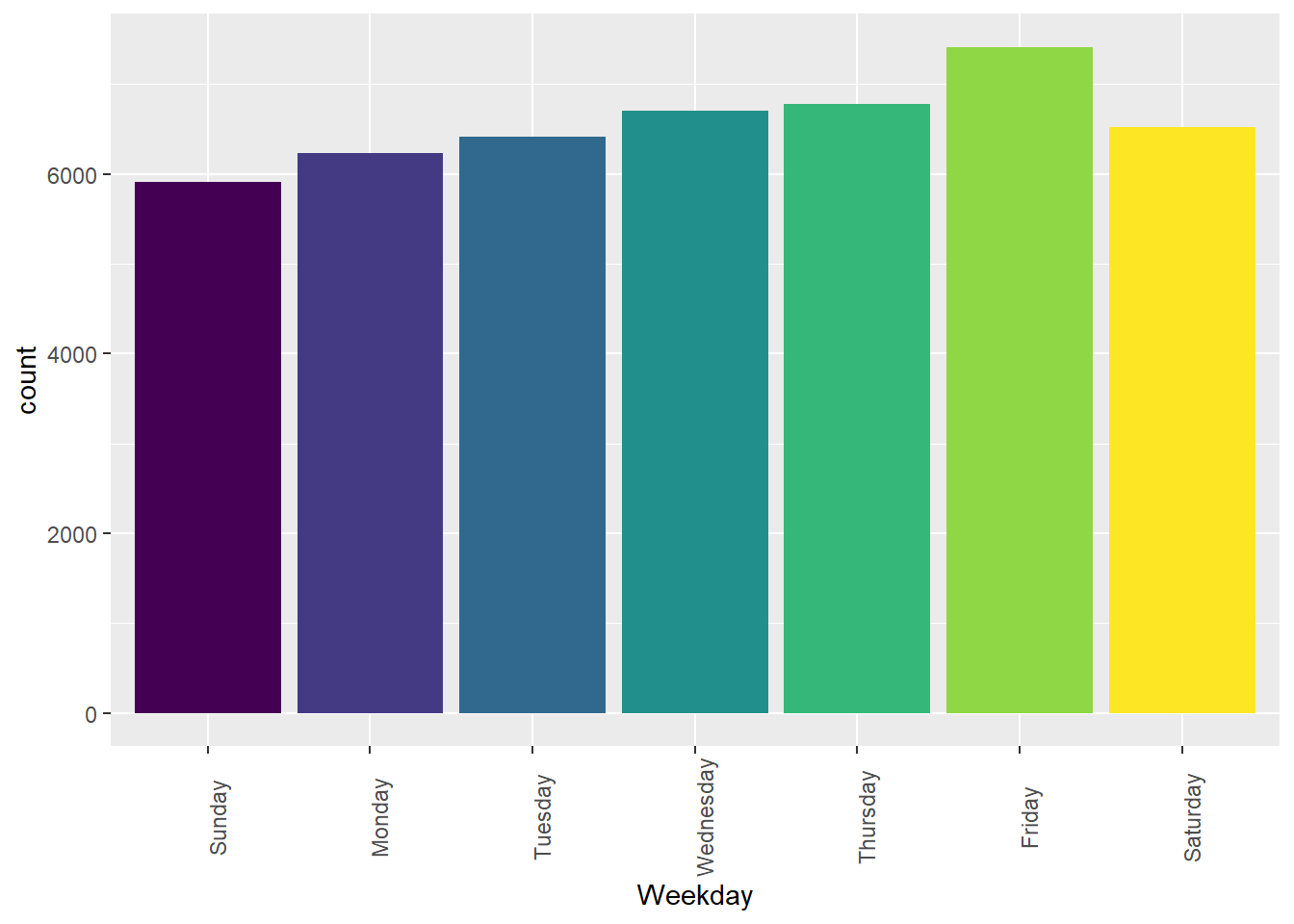
When subsetted for Crash Severity, however Boston sees the most fatal accidents on Wednesday and Saturday.
mydata %>%
  filter(Crash_Severity != "Unknown/Not Reported") %>%
ggplot(aes(Weekday, fill = Weekday)) +
  geom_bar( stat = "count") + facet_wrap ( ~ Crash_Severity, scales = "free_y") + theme(axis.text.x = element_text(angle = 90)) + theme(legend.position = "none")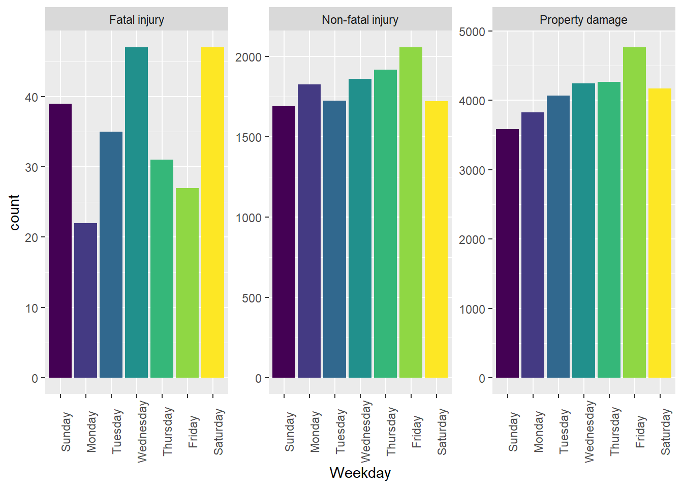
Crash Data by Month
Overall, October is the month with the highest Crash Ratings over 2012-2022. Let’s look at how each crash severity rating factors into overall highest crash ratings.
What could we learn about October? Are there significant events that happen in October? Is it all happening around Halloween? Or does weather condition have something to do with the increase in accidents?
#Crash Count per Day by Month
mydatamonthsum <- mydata %>%
  group_by(Month) %>%
  summarize("min" = min(Crash_Count, na.rm = TRUE),
            "max" = max(Crash_Count, na.rm = TRUE),
            "mean" = mean(Crash_Count, na.rm = TRUE),
            "median" = median(Crash_Count, na.rm = TRUE),
            "standard_deviation" = sd(Crash_Count, na.rm = TRUE))%>%
  arrange(Month)
mydatamonthsum %>%
print(n=12)
# A tibble: 12 × 6
Month min max mean median standard_deviation
<ord> <int> <int> <dbl> <dbl> <dbl>
1 Jan 1 26 12.7 12 4.56
2 Feb 1 37 12.6 12 4.74
3 Mar 1 27 12.4 12 4.48
4 Apr 1 26 12.2 12 4.17
5 May 1 28 13.2 13 4.50
6 Jun 1 26 13.5 13 4.35
7 Jul 1 32 13.2 13 4.60
8 Aug 3 22 12.5 12 3.64
9 Sep 2 28 13.4 13 4.27
10 Oct 2 34 15.1 14 5.74
11 Nov 1 31 13.9 13 5.40
12 Dec 1 25 13.3 13 4.38ggplot(mydata, aes(Month, stat="count")) + geom_bar() 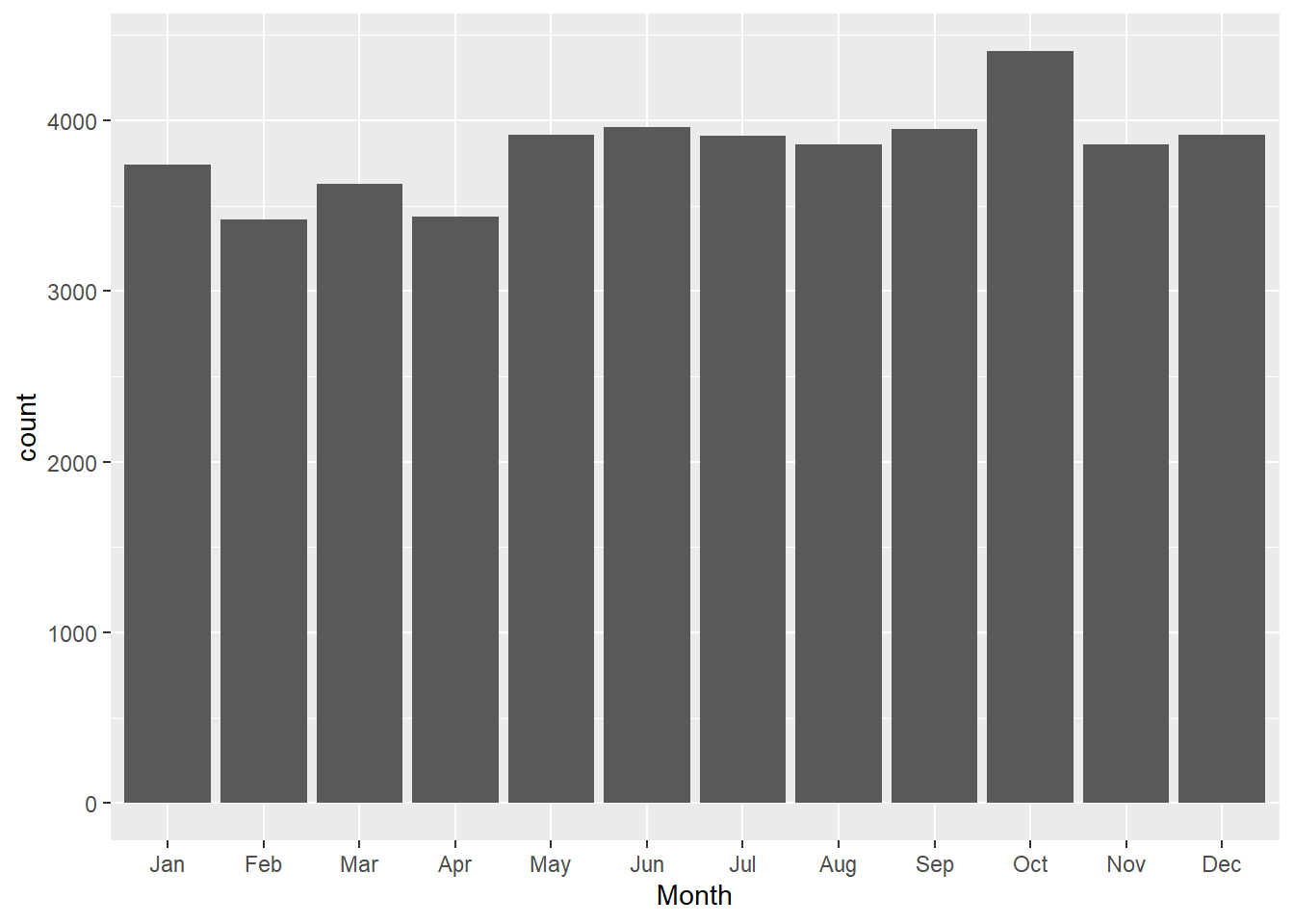
We can now see that the month with the highest Fatal injury is reported in July, with dips in spring, winter, and October while Non-fatal injuries and Property damage peak in October. The peak for Unknown/Not Reported crashes is in June and July.
ggplot(mydata, aes(Month, stat="count", fill = Crash_Severity)) + geom_bar() + facet_wrap( ~ Crash_Severity, scales = "free_y") + labs(title = "Crash Severity by Month (with free Y axis)") + theme(legend.position = "none")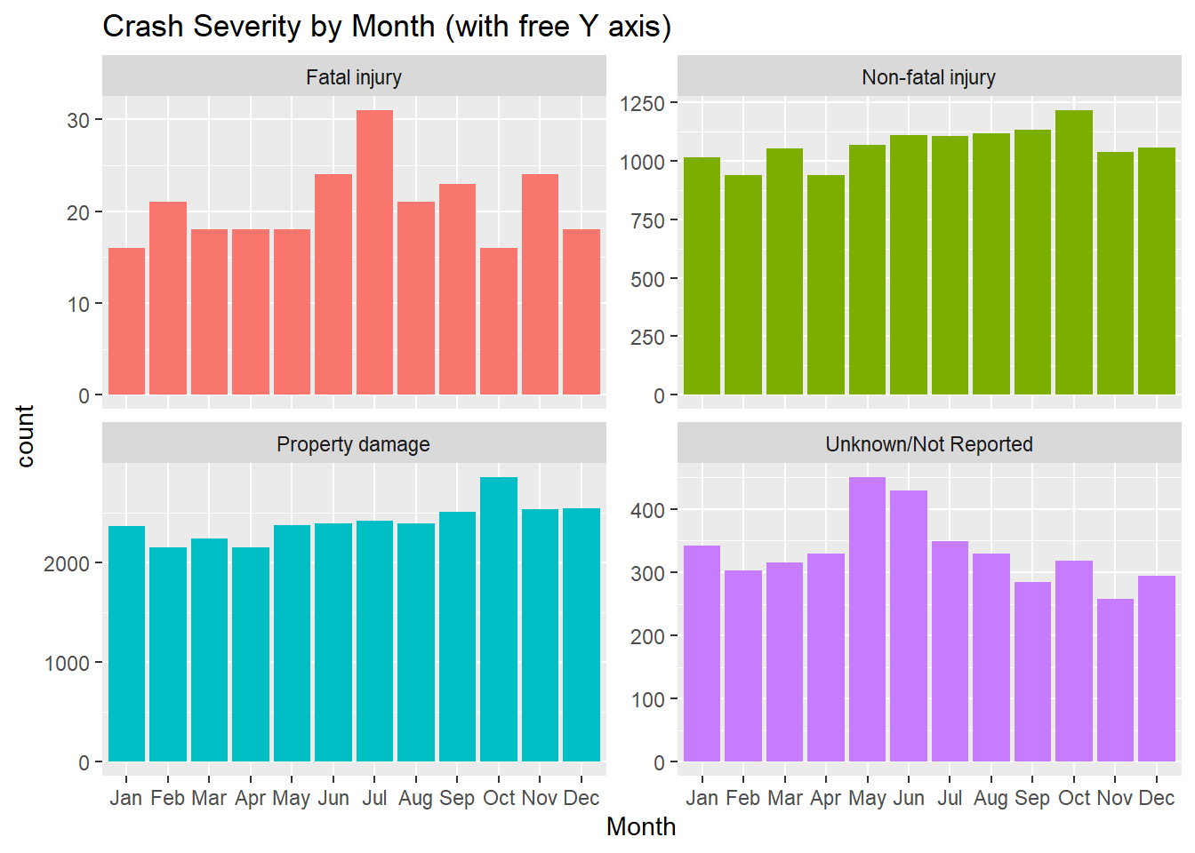
Crash Data by Year
Overall we see that 2017 was the year with the most Crashes from 2012-2022. The data shows 2017 as a peak with a sharp drop off in 2020 (due to the pandemic and reduced traffic flow) and a climb back up in 2021 almost matching crash reports from 2019. Of course this data shows that post-pandemic rates of car crashes has gone back up, but it is not as high as crashes in 2017. What happened in 2017 and were these crashes somehow different from crashes in 2016?
#Crash Count per Day by Year
mydatasum <- mydata %>%
  group_by(Year) %>%
  summarize("min" = min(Crash_Count, na.rm = TRUE),
            "max" = max(Crash_Count, na.rm = TRUE),
            "mean" = mean(Crash_Count, na.rm = TRUE),
            "median" = median(Crash_Count, na.rm = TRUE),
            "standard_deviation" = sd(Crash_Count, na.rm = TRUE)) %>%
  arrange(Year)

mydatasum %>%
print(n=11)
# A tibble: 11 × 6
Year min max mean median standard_deviation
<dbl> <int> <int> <dbl> <dbl> <dbl>
1 2012 1 26 12.5 12 4.41
2 2013 1 31 12.4 12 4.61
3 2014 2 29 12.8 12 4.78
4 2015 1 32 13.2 13 4.59
5 2016 1 34 13.2 13 4.44
6 2017 6 37 15.8 15 4.72
7 2018 1 28 14.6 14 4.44
8 2019 4 24 13.3 13 3.92
9 2020 1 29 10.6 10 4.45
10 2021 1 28 13.1 13 4.70
11 2022 2 26 12.0 12 4.37ggplot(mydata, aes(year(Crash_Date))) + geom_histogram(binwidth = .50) + scale_x_continuous(breaks=pretty_breaks())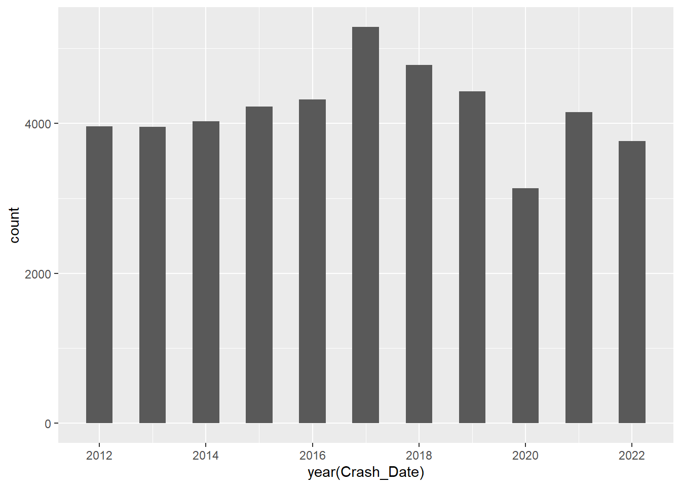
When yearly crash data is subset to look at Crash Severity we see different trends across the years. Fatal injury peaked in 2021 with 2016 close behind. Non-fatal injury peaked in 2017. Unknown/Not Reported crashes peaked in 2012 and in 2017. I wonder if in 2012 there was not an established standard to filling out reports and if in 2017 there were just more reports than could be fully processed.
ggplot(mydata, aes(Year, stat="count", fill = Crash_Severity)) + geom_bar() + scale_x_continuous(breaks=pretty_breaks()) +facet_wrap( ~ Crash_Severity, scales = "free_y" ) + labs(title = "Crash Severity by Year (with free Y axis)") + theme(legend.position = "none")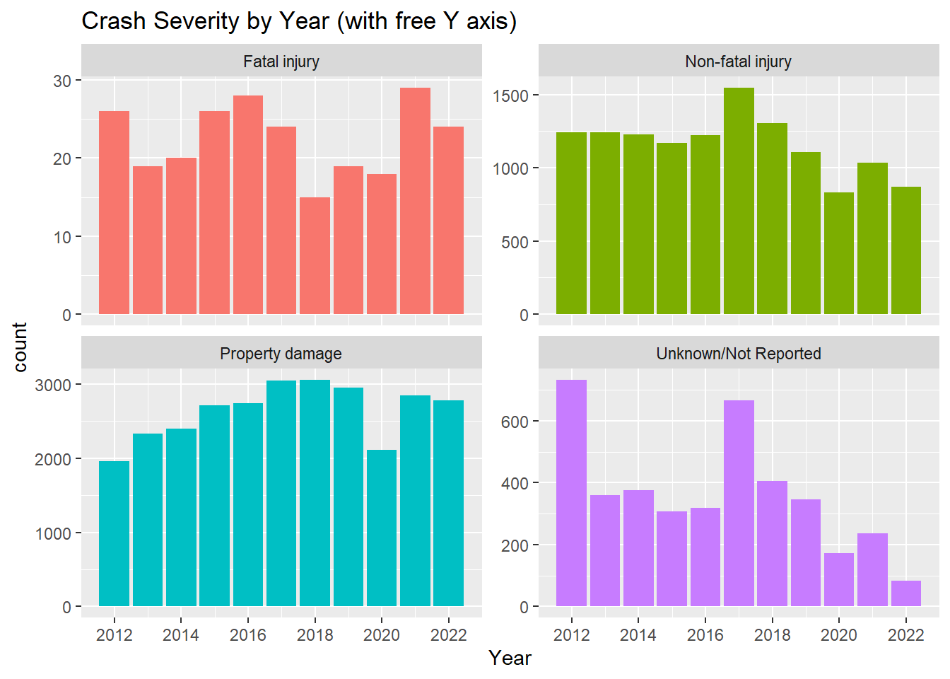
Crash Data by Time of Day
positions <- c("Morning", "Midday", "Afternoon", "Evening", "Late Night")

ggplot(mydata, aes(Crash_Time)) + geom_histogram()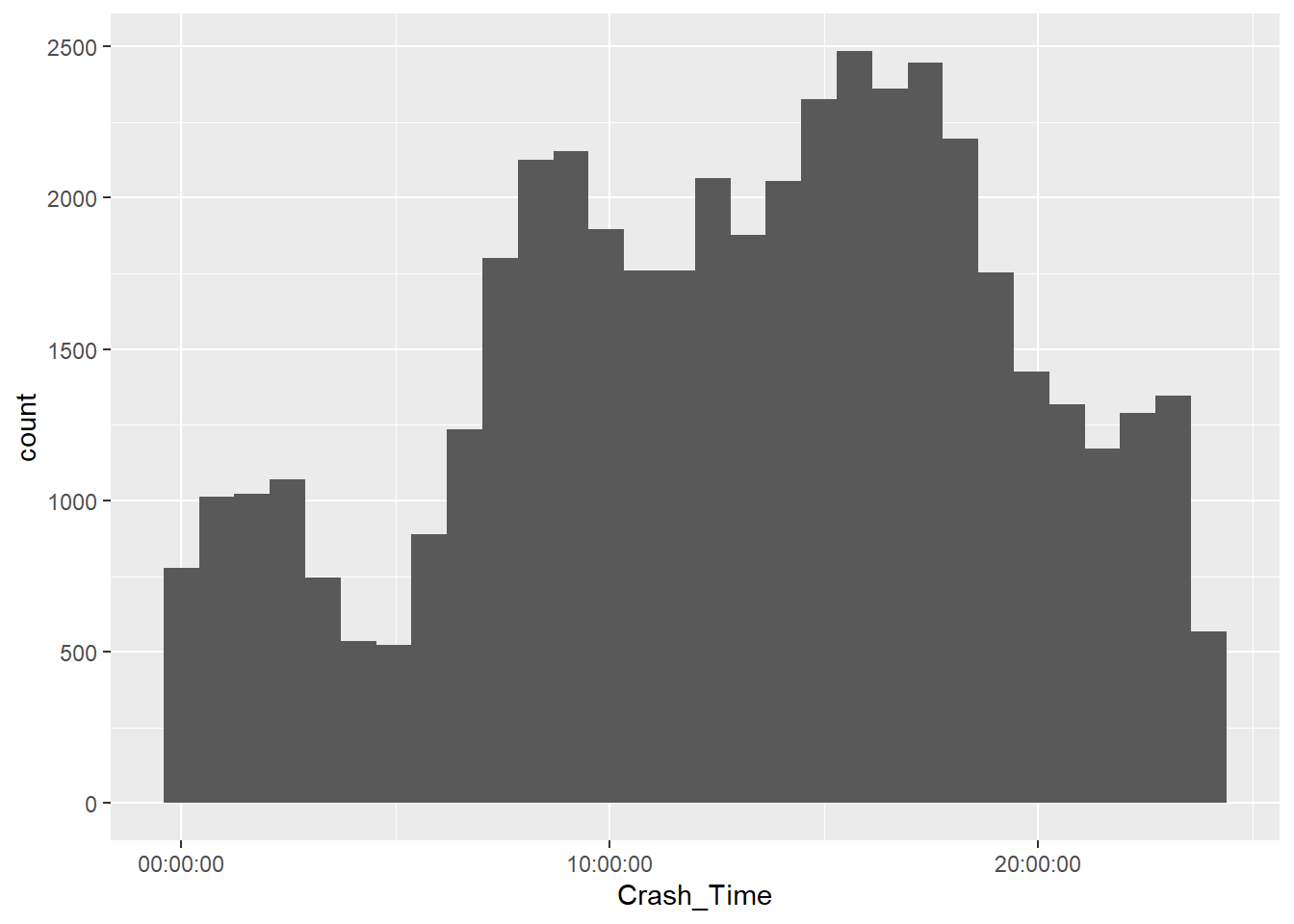
ggplot(mydata, aes(Crash_Time, stat="count", fill = Crash_Severity)) + geom_bar()+ theme(legend.position = "bottom")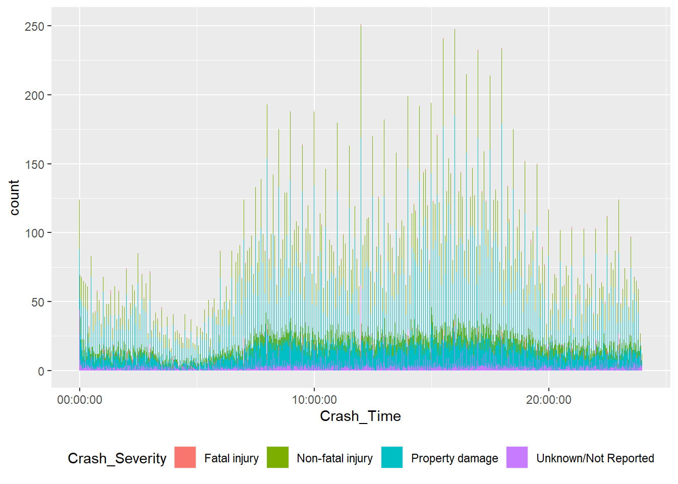
ggplot(mydata, aes(Crash_Time, stat="count", fill = Crash_Severity)) + geom_bar()+ theme(legend.position = "bottom") + facet_wrap ( ~ Crash_Severity, scales = "free_y") 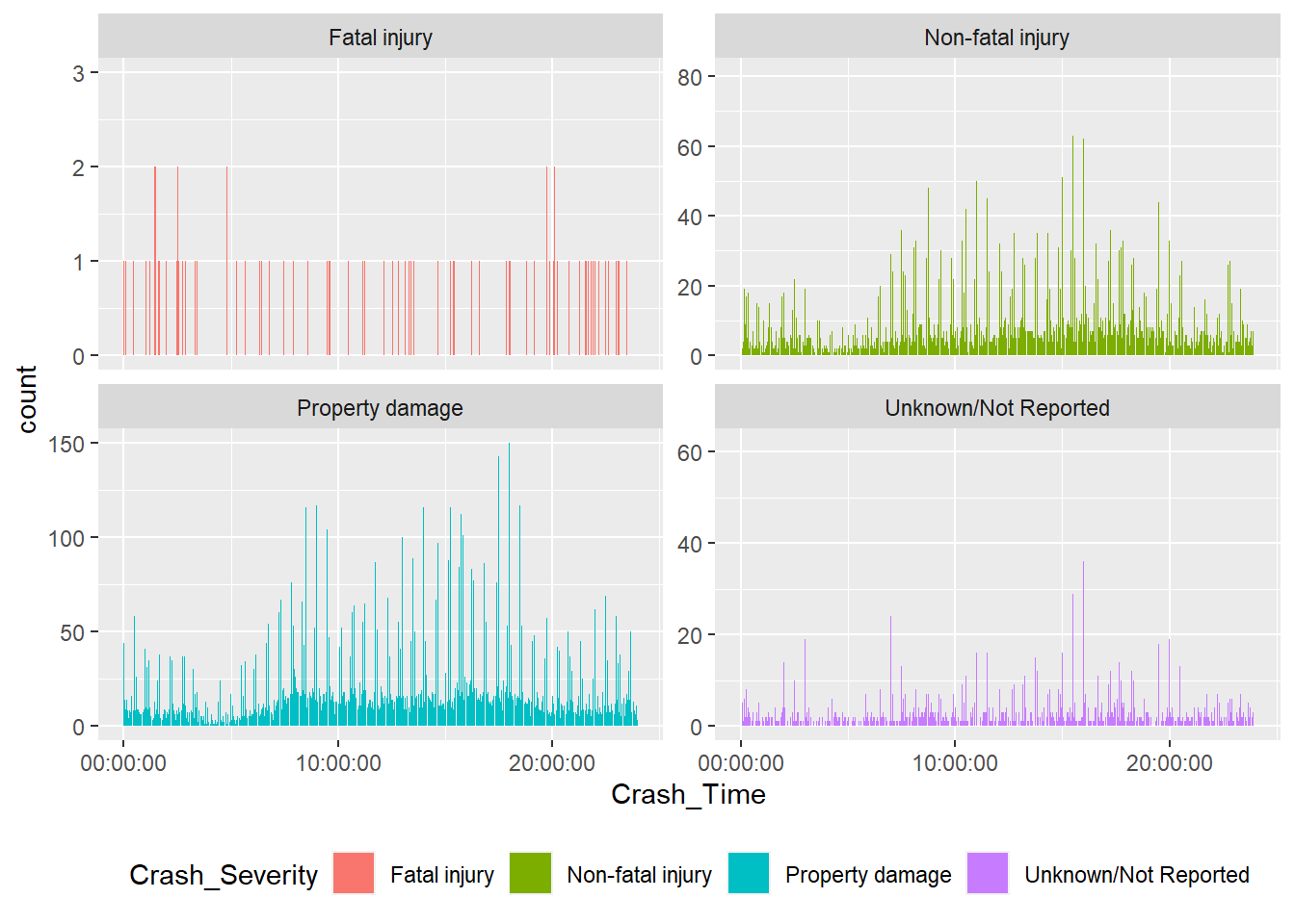
ggplot(mydata, aes(Crash_Timegroup, stat="count", fill = Crash_Severity)) + geom_bar() + scale_x_discrete(limits = positions)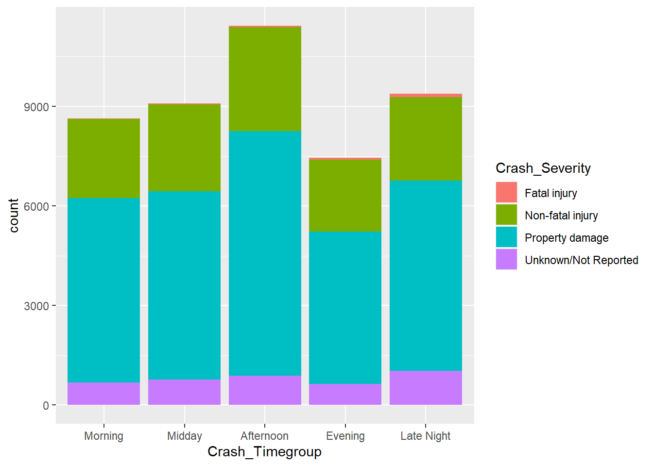
ggplot(mydata, aes(Crash_Timegroup, stat="count", fill = Crash_Severity)) + geom_bar() + facet_wrap ( ~ Crash_Severity, scales = "free_y") + scale_x_discrete(limits = positions) + theme(legend.position = "none")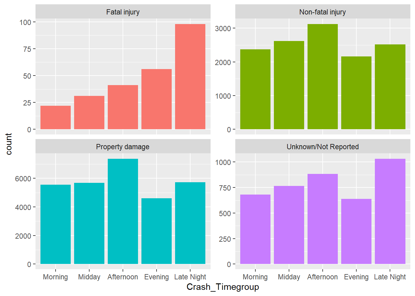
Crash Data by Manner of Collision
To no one’s surprise, we see that Rear-ends are the manner of collision that occurs most often in Boston. Following in second, third, and fourth respectively are: Single vehicle crashes,Angle crashes, and Sideswipe, same direction crashes.
positions2 <- c("Rear-end", "Single vehicle crash", "Angle", "Sideswipe, same direction", "Not reported", "Head-on", "Sideswipe, opposite direction", "Unknown", "Front to Rear", "Front to Front", "Rear-to-rear", "Rear to Side", "NA")

mydata %>%
  ggplot(., aes(x= Manner_of_Collision, stat = "count", fill = Manner_of_Collision)) +
geom_bar() + labs(title = "Manner of Collision from 2012-2022") + coord_flip() + theme(legend.position = "none") + scale_x_discrete(limits = positions2) 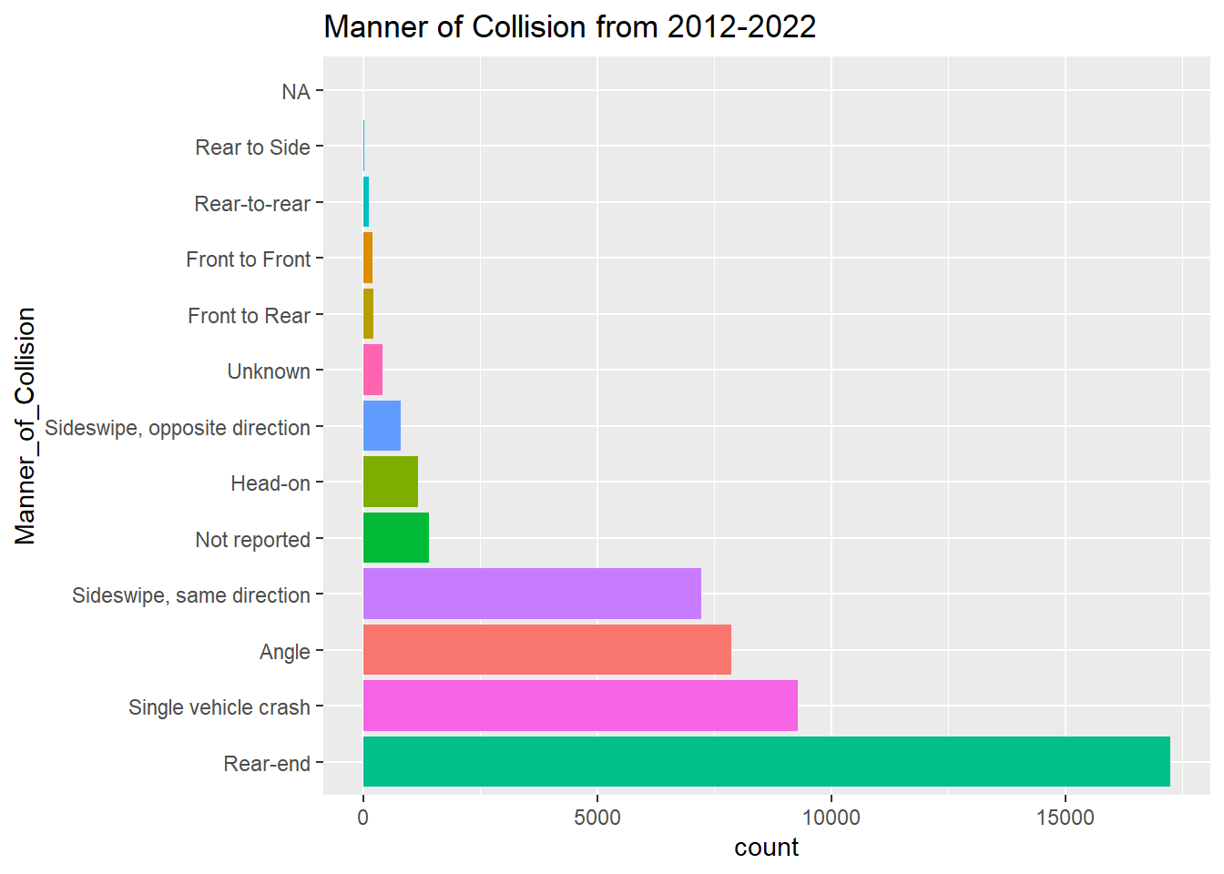
mydata %>%
  ggplot(aes(x= Manner_of_Collision, stat = "count", fill = Manner_of_Collision)) +
  geom_bar() +  labs(title = "Manner of Collision from 2012-2022, with free-x axis") + coord_flip() + theme(legend.position = "none") + facet_wrap ( ~ Crash_Severity, scales = "free_x") + scale_x_discrete(limits = positions2)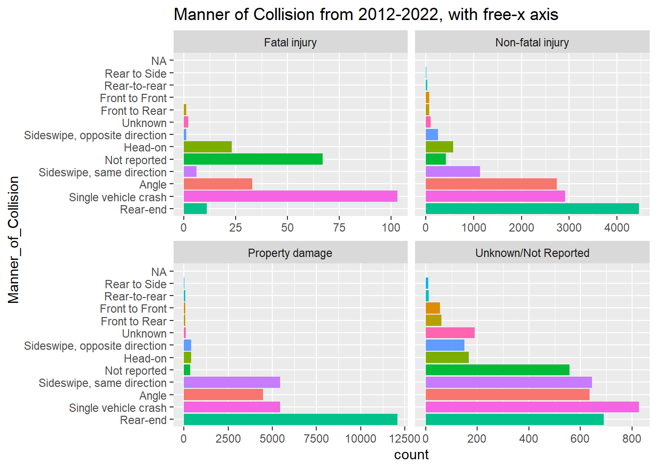
mydata %>%
  filter(Crash_Severity == "Fatal injury") %>%
  ggplot(aes(x= Manner_of_Collision, stat = "count", fill = Manner_of_Collision)) +
  geom_bar() +  labs(title = "Manner of Collision for Fatal Crashes from 2012-2022") + coord_flip() + theme(legend.position = "none")+ scale_x_discrete(limits = positions2)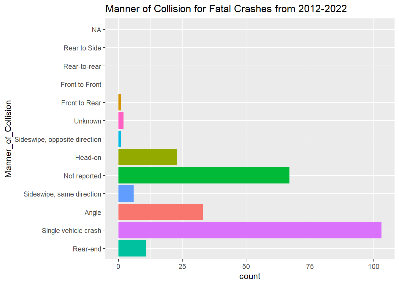
Part 4. Handling Unknown, Not Reported, NA or Missing data
Unknown and Not Reported incidents
All 46 reporting inconsistencies occurred between May 2018 and October 2019:
Crash Severity “Non-fatal injury” has 7 reports of “no injury” and just under 300 counts of “possible” or “suspected” injuries.
Crash Severity “Not Reported” has 42 reports of maximum injury reports across 6 categories that suggest a possible injury.
Crash Severity “Property damage” has 11 reports of a maximum injury reported as being “not reported”.
Crash Severity “Unknown” has 7 reports of non-fatal injury as either “Non-incapacitating” or “Possible”.
mydataog$Crash_Date <- as.Date(mydataog$Crash_Date, "%d-%b-%Y")
mydataog$Year <- year(mydataog$Crash_Date)

mydataog <- mydataog %>%
mutate(Crash_Severity = recode(Crash_Severity, `Property damage only (none injured)` = "Property damage"))
mydatainconsistencies <- mydataog %>%
  filter(between(Crash_Date, as.Date('2018-05-01'), as.Date('2019-10-31')))

tabinconsistencies <- table(mydatainconsistencies$Maximum_Injury_Severity_Reported, mydatainconsistencies$Crash_Severity) # Table for 2018-05-01:2019-10-31
tabinconsistencies
                                        Fatal injury Non-fatal injury
  Deceased not caused by crash                     0                3
  Fatal injury (K)                                30                0
  No Apparent Injury (O)                           0                0
  No injury                                        0                1
  Non-fatal injury - Incapacitating                0              142
  Non-fatal injury - Non-incapacitating            0              686
  Non-fatal injury - Possible                      0              455
  Not Applicable                                   0                0
  Not reported                                     0                0
  Possible Injury (C)                              0              238
  Suspected Minor Injury (B)                       0              273
  Suspected Serious Injury (A)                     0               18
  Unknown                                          0                0

                                        Not Reported Property damage Unknown
  Deceased not caused by crash                     1               0       0
  Fatal injury (K)                                 0               0       0
  No Apparent Injury (O)                          20            1786       1
  No injury                                       31            2766       3
  Non-fatal injury - Incapacitating                3               0       0
  Non-fatal injury - Non-incapacitating           14               0       3
  Non-fatal injury - Possible                     17               0       4
  Not Applicable                                  56               0       2
  Not reported                                   326               0     101
  Possible Injury (C)                              3               0       0
  Suspected Minor Injury (B)                       3               0       0
  Suspected Serious Injury (A)                     2               0       0
Unknown 0 0 21ggplot(mydataog, aes(x=Year, fill = Crash_Severity)) + geom_bar() + facet_wrap( ~ Crash_Severity, scales = "free_y") + theme(legend.position = "none") + scale_x_continuous(breaks=pretty_breaks()) 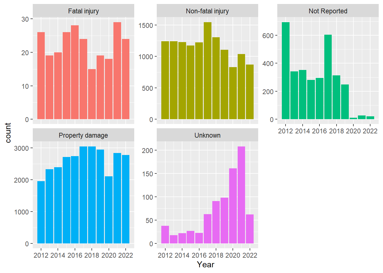
ggplot(mydata, aes(x=Year, fill = Crash_Severity)) + geom_bar() + facet_wrap( ~ Crash_Severity, scales = "free_y") + theme(legend.position = "none") + scale_x_continuous(breaks=pretty_breaks()) 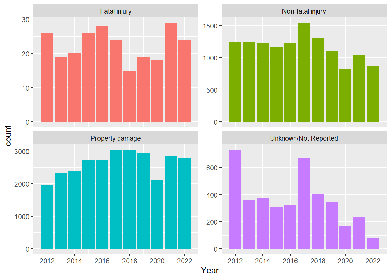
mydata %>%
  filter(Crash_Severity == "Unknown/Not Reported") %>%
  filter(between(Crash_Date, as.Date('2018-05-01'), as.Date('2019-10-31'))) %>%
ggplot(., aes(x=Maximum_Injury_Severity_Reported, stat="count", fill = Maximum_Injury_Severity_Reported)) + geom_bar() + coord_flip() + facet_wrap (~ Crash_Severity, scales = "free_x") + theme(legend.position = "none") +labs(title = str_wrap("Inconsistencies in Reported Crash Severity Between May 1st, 2018 and October 31st, 2019", width = 50))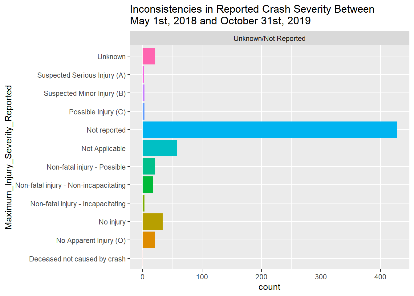
Missing data/NAs and outliers? And why do you choose this way to deal with NAs?
*should I fix the 20 data that report unknown or not reported for crash severity and then list either “Non-fatal injury - Incapacitating” or “Non-fatal injury - Non-incapacitating” in Maximum_Injury_Severity_Reported?*
sapply(mydata, function(x) sum(is.na(x))) Crash_Number
0
City_Town_Name
0
Crash_Date
0
Crash_Time
0
Crash_Severity
0
Maximum_Injury_Severity_Reported
0
Number_of_Vehicles
0
Total_Nonfatal_Injuries
0
Total_Fatal_Injuries
0
Manner_of_Collision
5
Vehicle_Action_Prior_to_Crash
8
Vehicle_Travel_Directions
4
Most_Harmful_Events
2639
Vehicle_Configuration
213
Road_Surface_Condition
368
Ambient_Light
1
Weather_Condition
0
At_Roadway_Intersection
33040
Distance_From_Nearest_Roadway_Intersection
309
Distance_From_Nearest_Milemarker
43298
Distance_From_Nearest_Exit
36521
Distance_From_Nearest_Landmark
35704
Non_Motorist_Type
43462
X_Cooordinate
1934
Y_Cooordinate
1934
Weekday
0
Month
0
Year
0
Crash_Hour
0
Crash_Timegroup
0
Crash_Count
0
Crash_Countgroup
0