In 2018, data was collected on the top 15 pathogens, which includes information on the total number of cases and the estimated cost associated with each pathogen.
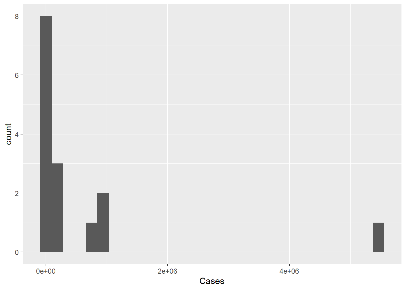
Due to the limited number of observations and highly skewed distribution of data, the feasibility of using similar visualizations as for a larger dataset or less skewed data needs to be evaluated, as we are dealing with only 15 observations, which is even fewer than the number of cereals in some datasets.
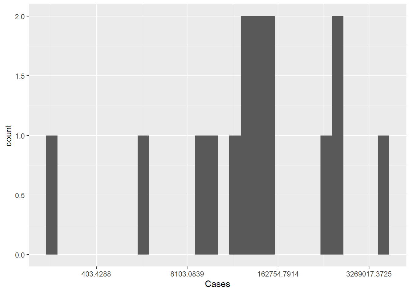
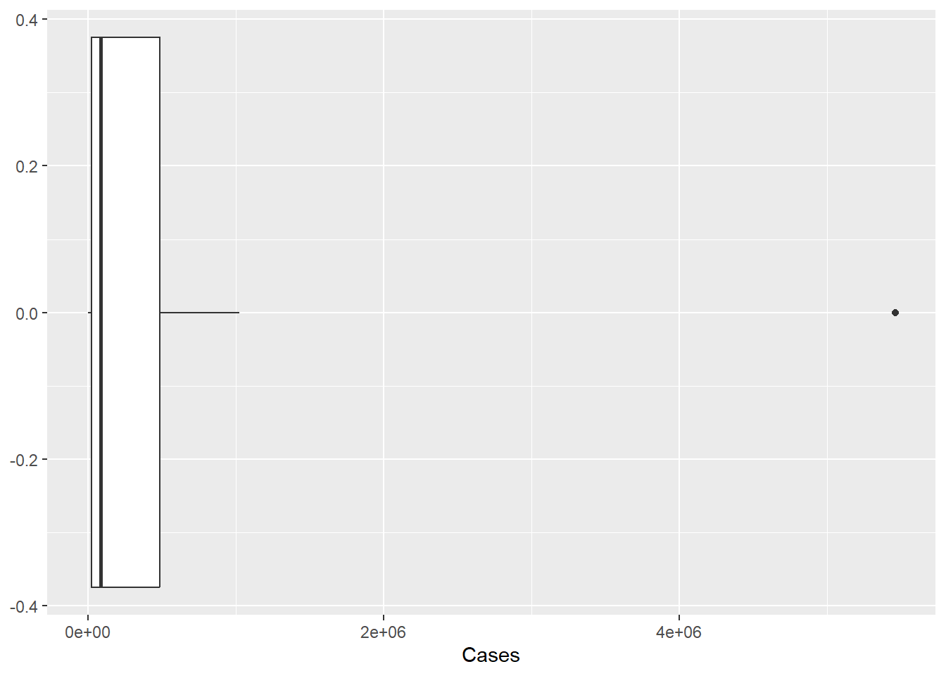
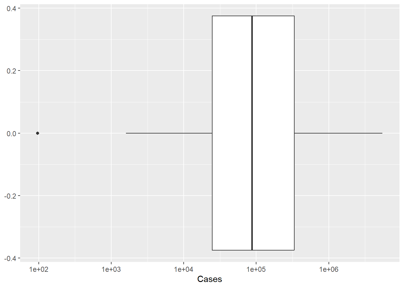
The histogram plot may not be the optimal choice for visualizing the distribution of the dataset, as it highlights the single outlier but may not provide enough insight into the cases of pathogens with lower counts. A suggestion was made to rescale the number of cases using a logarithmic or other scaling function to improve the visualization. As demonstrated in the subsequent plot, using a logarithmic scaling function for the x-axis has proven to be more informative in revealing the underlying patterns of the data.
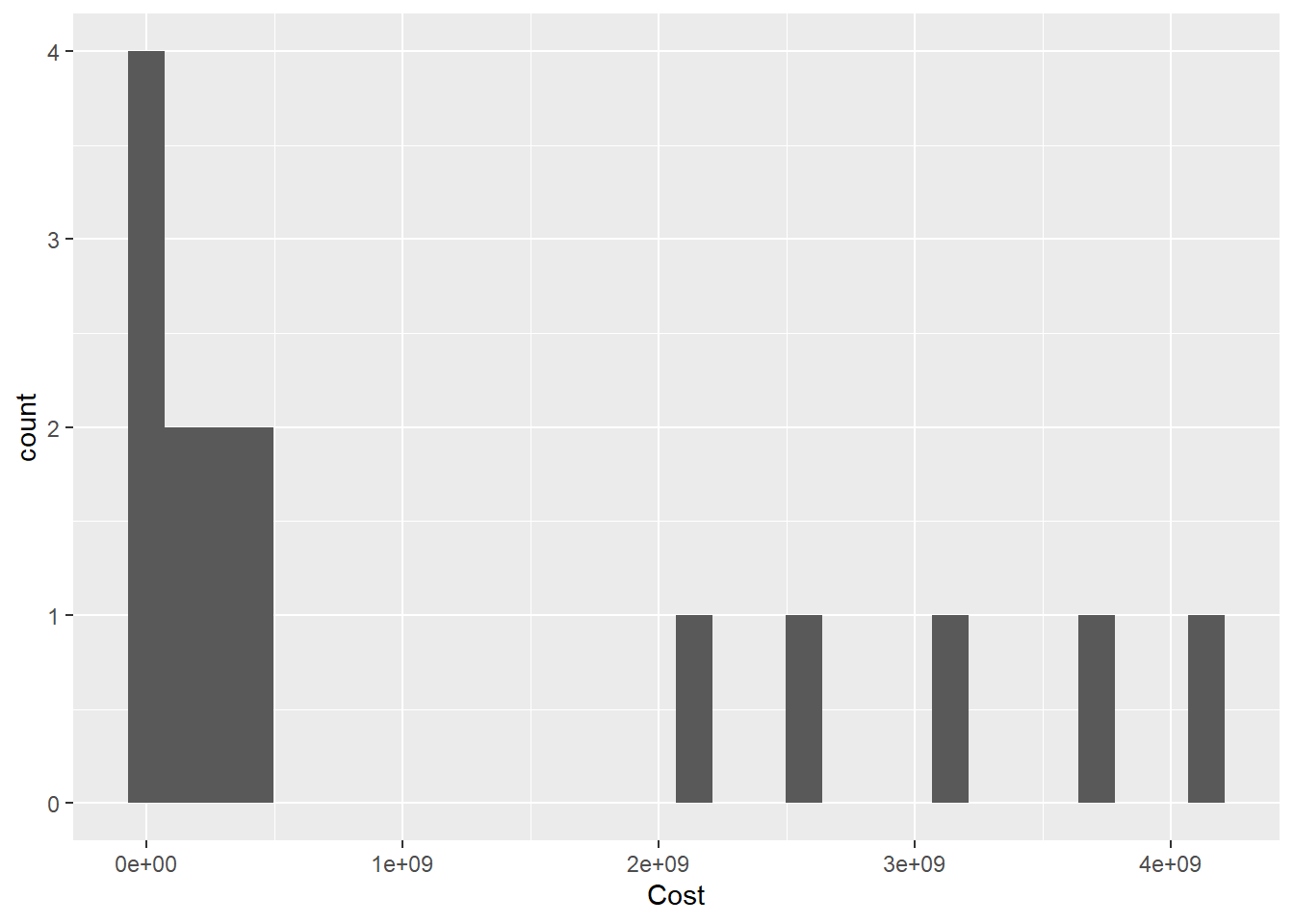
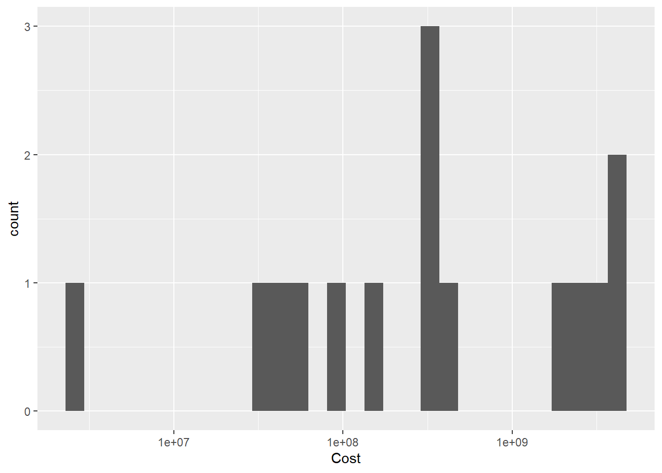
exploring the distribution of costs by plotting a graph.
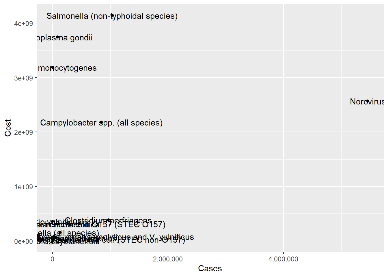
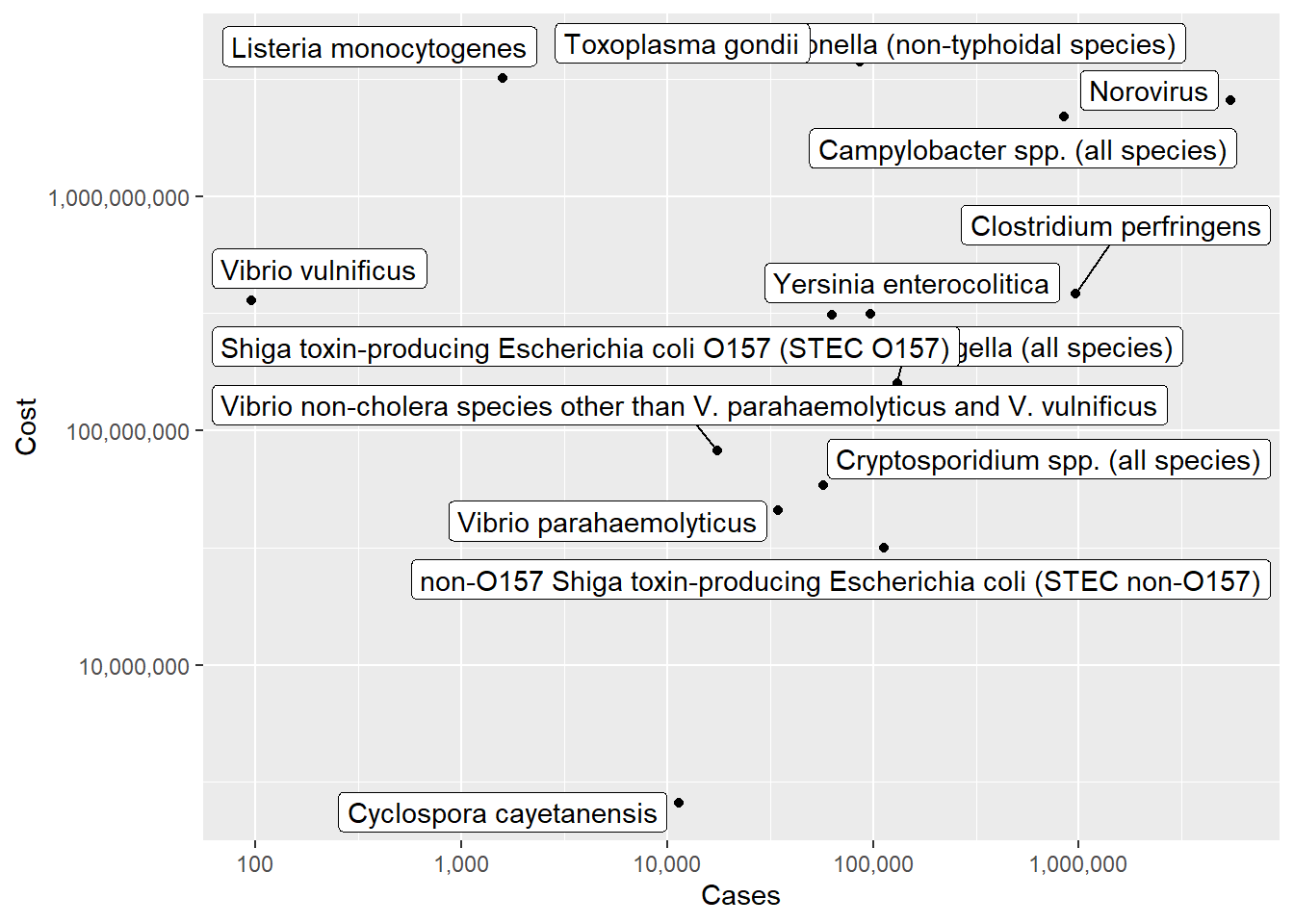
Although the logged and unlogged scatterplots provided some insight, the visualizations may not be particularly informative for a layperson. It is possible that the dataset would be better utilized by someone with expertise in this field, who can use it as a reference point.
Source Code
---title: "Challenge 5"author: "Thrishul"desription: "More data wrangling: pivoting"date: "03/22/2023"format: html: toc: true code-fold: true code-copy: true code-tools: truecategories: - challenge_5 - pathogen - cereal ---```{r}library(tidyverse)library(ggplot2)library(readxl)library(ggrepel)library(here)knitr::opts_chunk$set(echo =TRUE, warning=FALSE, message=FALSE)```In 2018, data was collected on the top 15 pathogens, which includes information on the total number of cases and the estimated cost associated with each pathogen.```{r}pathogen<-here("posts","_data","Total_cost_for_top_15_pathogens_2018.xlsx") %>% readxl::read_excel(skip=5, n_max=16, col_names =c("pathogens", "Cases", "Cost"))pathogen```### Univariate VisualizationsDue to the limited number of observations and highly skewed distribution of data, the feasibility of using similar visualizations as for a larger dataset or less skewed data needs to be evaluated, as we are dealing with only 15 observations, which is even fewer than the number of cereals in some datasets.```{r}ggplot(pathogen, aes(x=Cases)) +geom_histogram()ggplot(pathogen, aes(x=Cases)) +geom_histogram()+scale_x_continuous(trans ="log")ggplot(pathogen, aes(x=Cases)) +geom_boxplot()ggplot(pathogen, aes(x=Cases)) +geom_boxplot()+scale_x_continuous(trans ="log10")```The histogram plot may not be the optimal choice for visualizing the distribution of the dataset, as it highlights the single outlier but may not provide enough insight into the cases of pathogens with lower counts. A suggestion was made to rescale the number of cases using a logarithmic or other scaling function to improve the visualization. As demonstrated in the subsequent plot, using a logarithmic scaling function for the x-axis has proven to be more informative in revealing the underlying patterns of the data.## exploring the distribution of costs by plotting a graph.```{r}ggplot(pathogen, aes(x=Cost)) +geom_histogram()ggplot(pathogen, aes(x=Cost)) +geom_histogram()+scale_x_continuous(trans ="log10")```## Bivariate VisualizationTo further investigate the relationship between cases and costs, bivariate visualizations were created using both logged and unlogged scatterplots. ```{r}ggplot(pathogen, aes(x=Cases, y=Cost, label=pathogens)) +geom_point() +scale_x_continuous(labels = scales::comma)+geom_text()ggplot(pathogen, aes(x=Cases, y=Cost, label=pathogens)) +geom_point()+scale_x_continuous(trans ="log10", labels = scales::comma)+scale_y_continuous(trans ="log10", labels = scales::comma)+ ggrepel::geom_label_repel()```Although the logged and unlogged scatterplots provided some insight, the visualizations may not be particularly informative for a layperson. It is possible that the dataset would be better utilized by someone with expertise in this field, who can use it as a reference point.