read in a data set, and describe the data set using both words and any supporting information (e.g., tables, etc)
tidy data (as needed, including sanity checks)
mutate variables as needed (including sanity checks)
Recreate at least two graphs from previous exercises, but introduce at least one additional dimension that you omitted before using ggplot functionality (color, shape, line, facet, etc) The goal is not to create unneeded chart ink (Tufte), but to concisely capture variation in additional dimensions that were collapsed in your earlier 2 or 3 dimensional graphs.
Explain why you choose the specific graph type
If you haven’t tried in previous weeks, work this week to make your graphs “publication” ready with titles, captions, and pretty axis labels and other viewer-friendly features
R Graph Gallery is a good starting point for thinking about what information is conveyed in standard graph types, and includes example R code. And anyone not familiar with Edward Tufte should check out his fantastic books and courses on data visualizaton.
(be sure to only include the category tags for the data you use!)
Read in data
Read in one (or more) of the following datasets, using the correct R package and command.
Generated by summarytools 1.0.1 (R version 4.2.2) 2023-05-22
Briefly describe the data
We can see there are lots of attributes in these dataset.There are 32 attributes and 119390 rows.For challenge 6 I mainly focus on date and different kind of customers.
Firstly,I transfer string type of month to int for combine year and month,thus more convenient to observe the relationship between the total number of guests of each month and time.
   Min. 1st Qu.  Median    Mean 3rd Qu.    Max.
  0.000   2.000   2.000   1.968   2.000  55.000
Time Dependent Visualization
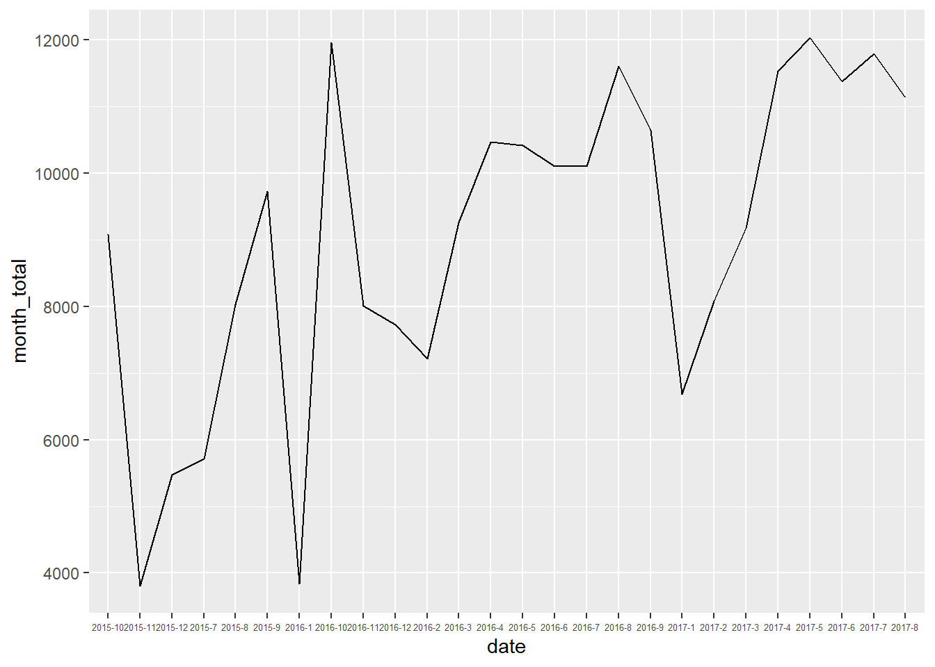
According to the date column I processed previously,I grouped the rows by month and use summarise() to calculate the total guests number of each month from 2015 to 2017.
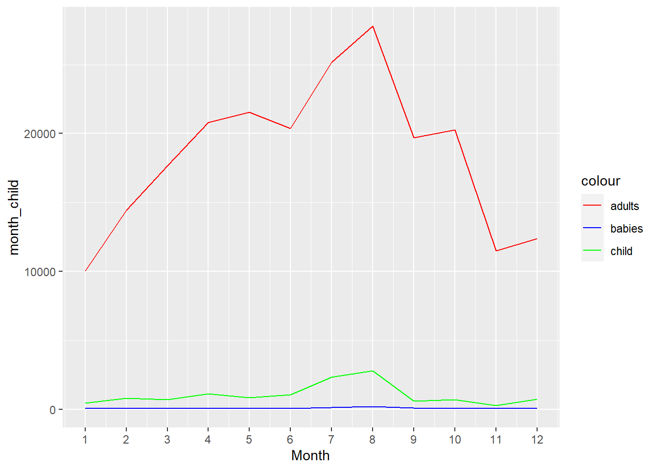
In challenge 6, I explored the relationship between months and different type of guests. Firstly I calculated the total monthly amount of different kinds of guests separately.
Then I drawed lines for each kind of guests:adults,child and babies. I find that there are many more adult guests than children and babies!And almost all year round at a very high level except from November to January it may means people will travel less in winter. For children,although the number of children is very low,but what is interesting is that during the summer holidays (June to September) there is a significant increase.It can be seen that children usually go out in the summer holidays. As for babies, the number of hotel reservations has remained at a very low number.
ggplot(hotel_type, aes(Month,month_child,group =1,col ="child")) +geom_line() +geom_line(aes(Month,month_babies, group =1,col ="babies")) +geom_line(aes(Month,month_adults, group =1,col ="adults")) +scale_x_continuous(breaks =seq(1,12,1)) +scale_color_manual(values =c("red","blue","green"))
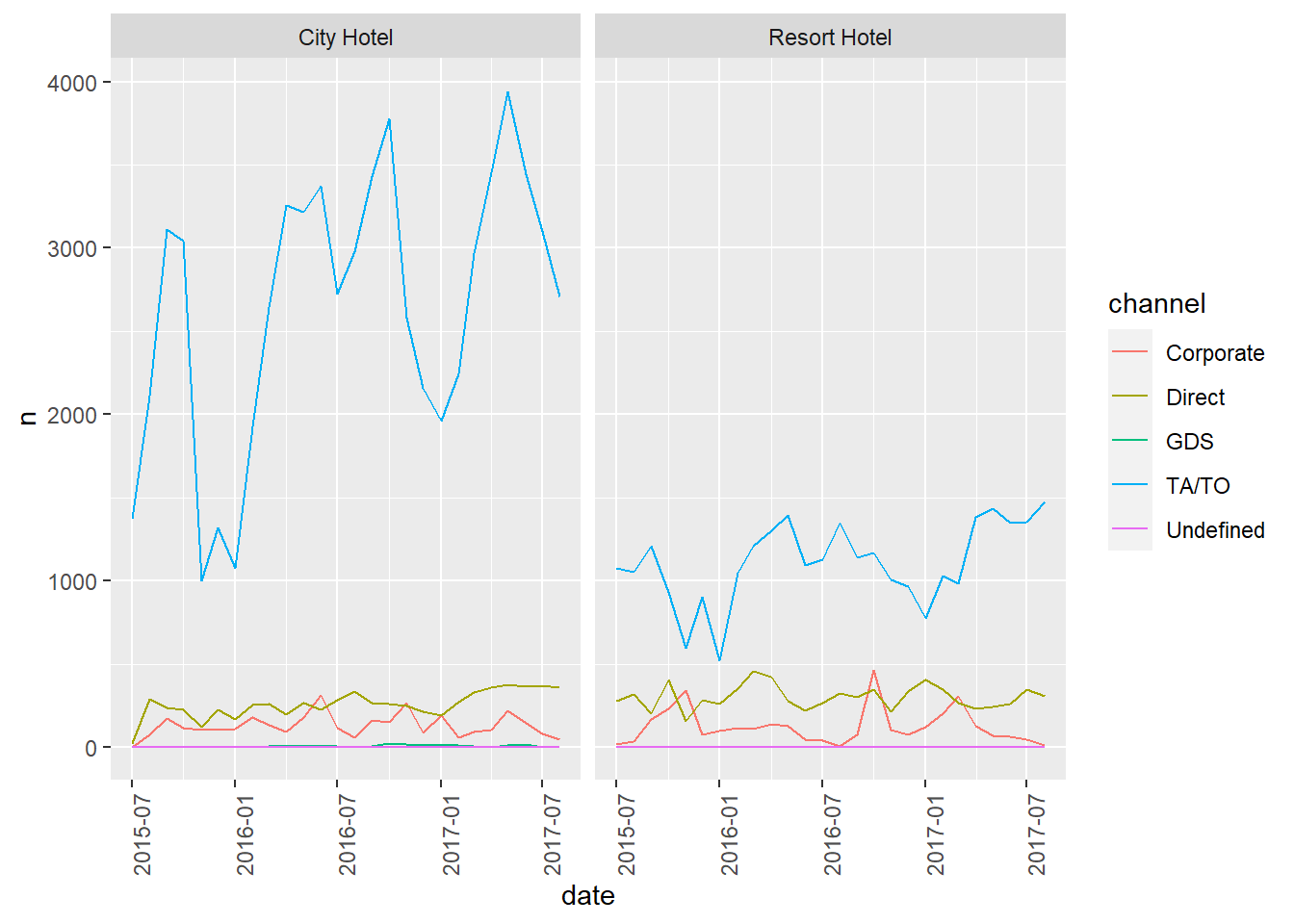
In challenge7,I’ll split the data base on distribution channel attribute. Firstly,to make the drawing easier,I’ll change the date type from chr to date.
        date        hotel   channel    n
1 2015-07-01   City Hotel Corporate    0
2 2015-07-01   City Hotel    Direct   27
3 2015-07-01   City Hotel       GDS    0
4 2015-07-01   City Hotel     TA/TO 1371
5 2015-07-01   City Hotel Undefined    0
6 2015-07-01 Resort Hotel Corporate   22
Now we can see the comparison of these 5 different channels in these 2 different hotel types.
ggplot(bookings_channel,aes(date, n, col=channel))+geom_line()+facet_wrap(vars(hotel))+scale_x_date()+theme(axis.text.x=element_text(angle=90))
Source Code
---title: "Challenge_7"author: "Xinyang Mao"description: "Visualizing Multiple Dimensions"date: "05/10/2023"format: html: toc: true code-copy: true code-tools: truecategories: - challenge_7 - hotel_bookings---```{r}#| label: setup#| warning: false#| message: falselibrary(tidyverse)library(ggplot2)library(lubridate)knitr::opts_chunk$set(echo =TRUE, warning=FALSE, message=FALSE)```## Challenge OverviewToday's challenge is to:1) read in a data set, and describe the data set using both words and any supporting information (e.g., tables, etc)2) tidy data (as needed, including sanity checks)3) mutate variables as needed (including sanity checks)4) Recreate at least two graphs from previous exercises, but introduce at least one additional dimension that you omitted before using ggplot functionality (color, shape, line, facet, etc) The goal is not to create unneeded [chart ink (Tufte)](https://www.edwardtufte.com/tufte/), but to concisely capture variation in additional dimensions that were collapsed in your earlier 2 or 3 dimensional graphs. - Explain why you choose the specific graph type5) If you haven't tried in previous weeks, work this week to make your graphs "publication" ready with titles, captions, and pretty axis labels and other viewer-friendly features[R Graph Gallery](https://r-graph-gallery.com/) is a good starting point for thinking about what information is conveyed in standard graph types, and includes example R code. And anyone not familiar with Edward Tufte should check out his [fantastic books](https://www.edwardtufte.com/tufte/books_vdqi) and [courses on data visualizaton.](https://www.edwardtufte.com/tufte/courses)(be sure to only include the category tags for the data you use!)## Read in dataRead in one (or more) of the following datasets, using the correct R package and command. - eggs ⭐ - abc_poll ⭐⭐ - australian_marriage ⭐⭐ - hotel_bookings ⭐⭐⭐ - air_bnb ⭐⭐⭐ - us_hh ⭐⭐⭐⭐ - faostat ⭐⭐⭐⭐⭐```{r}hotel_raw <-read.csv("_data/hotel_bookings.csv")print(summarytools::dfSummary(hotel_raw,varnumbers =FALSE,plain.ascii =FALSE, style ="grid", graph.magnif =0.70, valid.col =FALSE),method ='render',table.classes ='table-condensed')```### Briefly describe the dataWe can see there are lots of attributes in these dataset.There are 32 attributes and 119390 rows.For challenge 6 I mainly focus on date and different kind of customers.```{r}str(hotel_raw)```## Tidy DataFirstly,I transfer string type of month to int for combine year and month,thus more convenient to observe the relationship between the total number of guests of each month and time.```{r}hotel_raw<-na.omit(hotel_raw)hotel <- hotel_raw%>%mutate(Month =match(arrival_date_month,month.name))head(hotel$Month)```Combine year and month used to display the graph later.```{r}hotel1 <- hotel%>%mutate(date =str_c(arrival_date_year,Month,sep ="-"))```check the result,it's what I want!```{r}head(hotel1$date)```Calculate the total number of guests for each day.```{r}hotel_month <- hotel1%>%mutate(total_guests =rowSums(select(.,adults,children,babies),na.rm =TRUE))summary(hotel_month$total_guests)```## Time Dependent VisualizationAccording to the `date` column I processed previously,I grouped the rows by month and use `summarise()` to calculate the total guests number of each month from 2015 to 2017.```{r}hotel_month<-hotel_month%>%group_by(date) %>%summarise(month_total =sum(total_guests)) %>%ungroup() %>%mutate(month_total =as.integer(month_total))hotel_month```Then draw a gragh for observing,we can see it was floated a lot,and the least crowded months are November 2015,Jan of both 2016 and 2017.```{r}ggplot(hotel_month, aes(x = date, y = month_total,group =1)) +geom_line() +theme(axis.text.x =element_text(size =5 ))```## Visualizing Part-Whole RelationshipsIn challenge 6, I explored the relationship between months and different type of guests.Firstly I calculated the total monthly amount of different kinds of guests separately.```{r}hotel_type<-hotel1%>%group_by(Month) %>%summarise(month_child =sum(children),month_babies =sum(babies),month_adults =sum(adults)) %>%ungroup() %>%mutate(month_child =as.integer(month_child),month_babies =as.integer(month_babies),month_adults =as.integer(month_adults),Month =month(Month))hotel_type```Then I drawed lines for each kind of guests:adults,child and babies.I find that there are many more adult guests than children and babies!And almost all year round at a very high level except from November to January it may means people will travel less in winter.For children,although the number of children is very low,but what is interesting is that during the summer holidays (June to September) there is a significant increase.It can be seen that children usually go out in the summer holidays.As for babies, the number of hotel reservations has remained at a very low number.```{r}ggplot(hotel_type, aes(Month,month_child,group =1,col ="child")) +geom_line() +geom_line(aes(Month,month_babies, group =1,col ="babies")) +geom_line(aes(Month,month_adults, group =1,col ="adults")) +scale_x_continuous(breaks =seq(1,12,1)) +scale_color_manual(values =c("red","blue","green"))theme(axis.text.x =element_text(size =2 ))```## Visualization with Multiple DimensionsIn challenge7,I'll split the data base on distribution channel attribute.Firstly,to make the drawing easier,I'll change the `date` type from `chr` to `date`.```{r}hotel_date <- hotel1hotel_date$date <-as.Date(paste0(hotel_date$date,'-1'),format='%Y-%m-%d')head(hotel_date$date)```Count the amount of each distribution channel type.```{r}count(hotel_date,distribution_channel)```We can see there are 5 types of distribution channel,I'd like to recode them as a new attribute `channel`.```{r}bookings_channel <- hotel_date %>%mutate(channel=recode(distribution_channel,Cor="Corporate",Dir="Direct",GDS="GDS",TT="TA/TO"),Un="Undefined",across(c(hotel, channel),as.factor)) %>%count(date, hotel, channel,.drop=F)``````{r}head(bookings_channel)```Now we can see the comparison of these 5 different channels in these 2 different hotel types.```{r}ggplot(bookings_channel,aes(date, n, col=channel))+geom_line()+facet_wrap(vars(hotel))+scale_x_date()+theme(axis.text.x=element_text(angle=90))```