Generated by summarytools 1.0.1 (R version 4.2.2) 2023-04-23
The AB_NYC_2019 dataset describes listing activities of Airbnb properties in different boroughs of New York City, in New York for 2019. Each row contains the name of the listings, id, name of the host as well as information on rental types, geographical coordinates, prices, reviews and their availability in 2019.
Tidy Data
I want to plot relationships between the date of review and other variables.The variable last_review contains missing values. So I first retain observations that were reviewed. Then, I create month and year columns from the date variable.
After this, I select a subset of variables.
mydata2 <- mydata %>%mutate(Date =ymd(last_review))%>%drop_na(Date)%>%mutate(day =day(Date), month =month(Date, label=TRUE), year =year(Date))#I first select the required variables.select_df<-mydata2 %>%select(id, neighbourhood_group:year)
I obtain the average number of reviews, and then only retain the listings that have number of reviews that are equal or higher than the average. Then I first group them by month and then by room type and month.
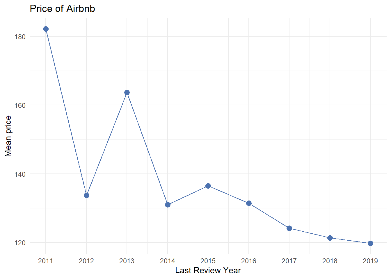
The graph shows how the price in 2019 varies with the month of review.
ggplot(summary_stats_month2, aes(x =as.integer(year), y = Mean, group=1)) +geom_line(color ="#4C72B0") +geom_point(size =3, color ="#4C72B0") +labs(title ="Price of Airbnb",x ="Last Review Year", y ="Mean price") +scale_x_continuous(breaks =seq(min(as.integer(summary_stats_month2$year)), max(as.integer(summary_stats_month2$year)), by =1),labels =seq(min(as.integer(summary_stats_month2$year)), max(as.integer(summary_stats_month2$year)), by =1)) +theme_minimal()
Time dependent visualization with different categories:
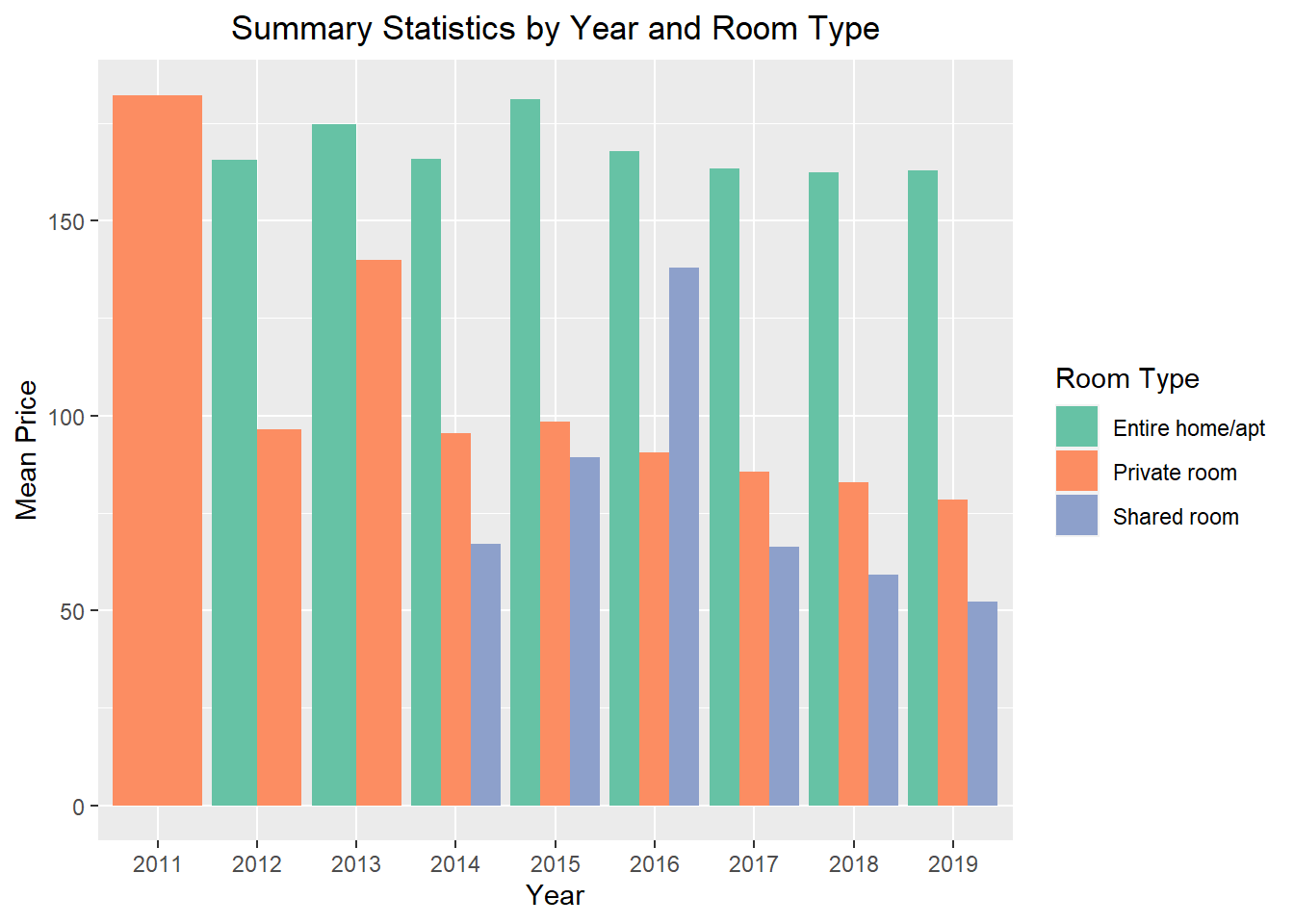
ggplot(summary_stats_month3, aes(x =factor(year), y = Mean, fill = room_type)) +geom_bar(stat ="identity", position =position_dodge(width =0.9)) +labs(x ="Year", y ="Mean Price", fill ="Room Type") +ggtitle("Summary Statistics by Year and Room Type") +theme(plot.title =element_text(hjust =0.5)) +scale_fill_brewer(palette ="Set2")
We can see that most recently reviewed airbnbs are cheaper compared to the ones that were last reviewed much before. One interesting pattern is the introduction of shared rooms that are much cheaper.
Continuing to play around
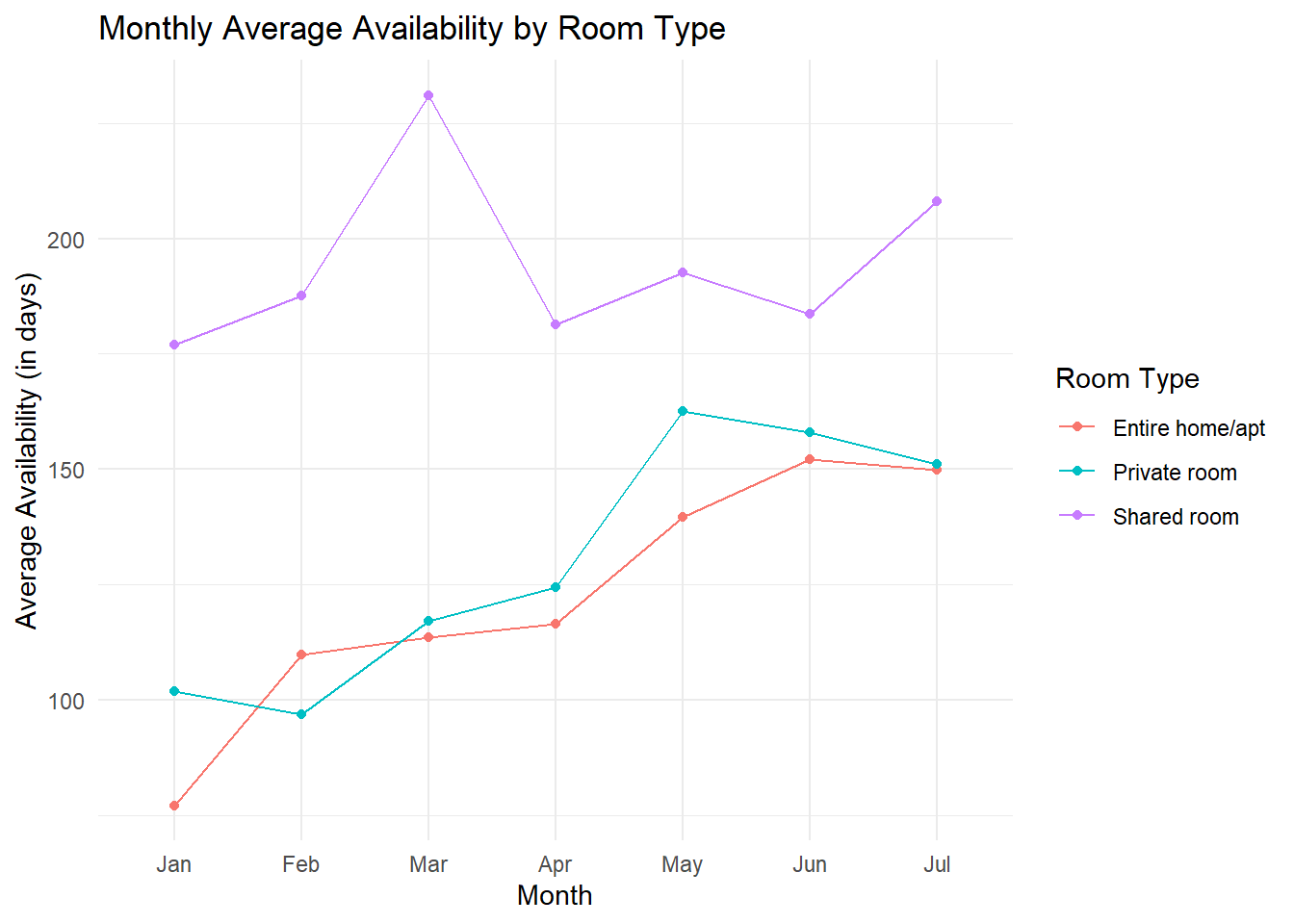
Next, I look at average availability for 2019, but I also take the type of listings into consideration:
select_df_type <- select_df %>%filter(year>=2019)%>%group_by(month, room_type) %>%summarise(count=n(), mean_availability=mean(availability_365)) %>%ungroup()ggplot(select_df_type, aes(x = month, y = mean_availability, color = room_type, group = room_type)) +geom_line() +geom_point() +labs(title ="Monthly Average Availability by Room Type",x ="Month",y ="Average Availability (in days)",color ="Room Type") +scale_color_manual(values =c("#F8766D", "#00BFC4", "#C77CFF")) +theme_minimal()
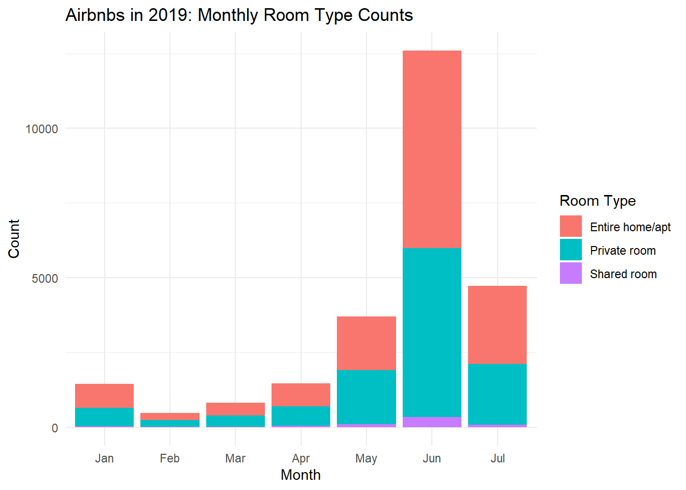
ggplot(select_df_type, aes(x = month, y = count, fill = room_type)) +geom_bar(stat ="identity", position ="stack") +labs(title ="Airbnbs in 2019: Monthly Room Type Counts",x ="Month",y ="Count",fill ="Room Type") +scale_fill_manual(values =c("#F8766D", "#00BFC4", "#C77CFF")) +theme_minimal()
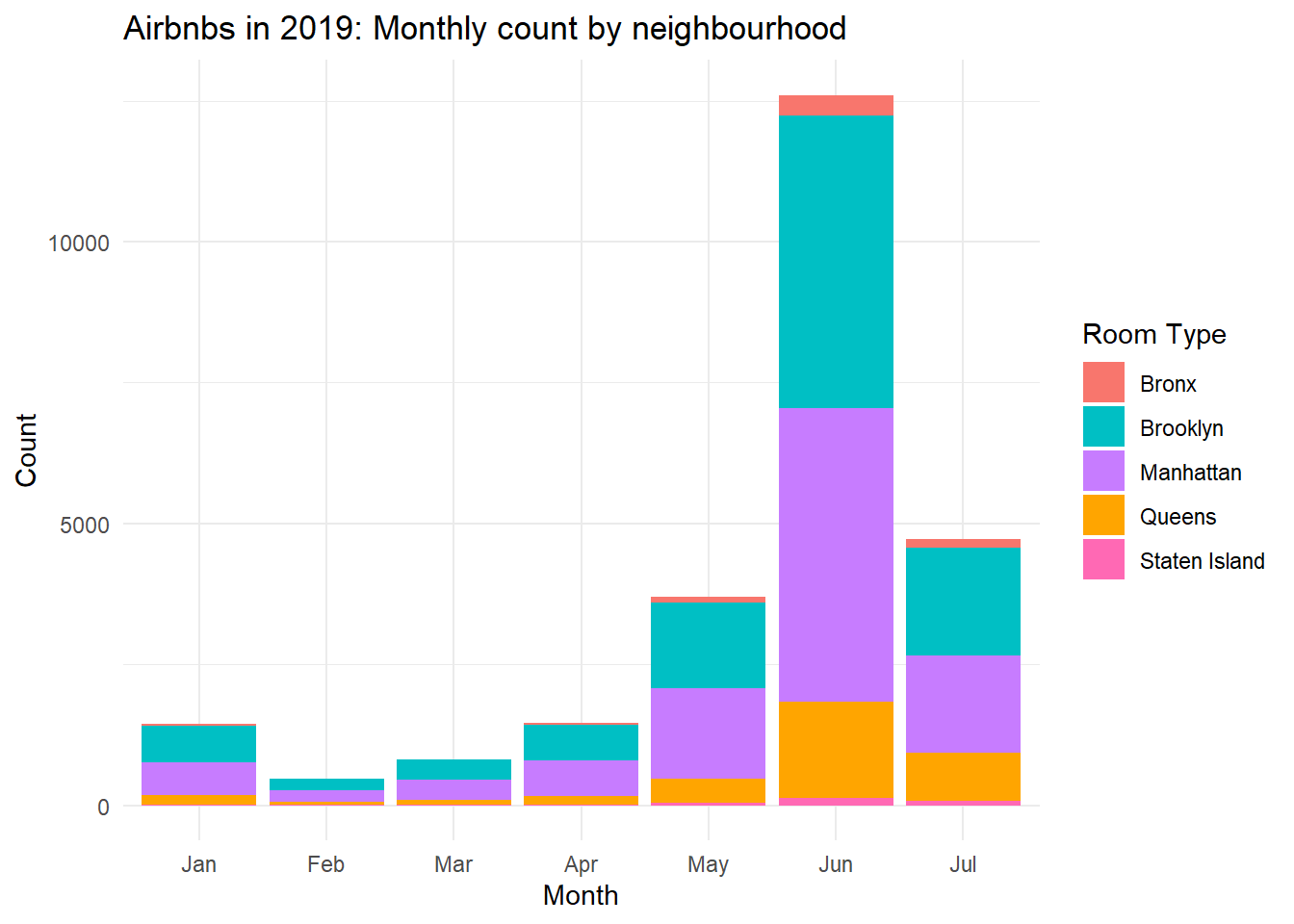
Looking at availability by neighbourhood:
select_df_type2 <- select_df %>%filter(year>=2019)%>%group_by(month, neighbourhood_group ) %>%summarise(count=n(), mean_availability=mean(availability_365)) %>%ungroup()ggplot(select_df_type2, aes(x = month, y = count, fill = neighbourhood_group)) +geom_bar(stat ="identity", position ="stack") +labs(title ="Airbnbs in 2019: Monthly count by neighbourhood",x ="Month",y ="Count",fill ="Room Type") +scale_fill_manual(values =c("#F8766D", "#00BFC4", "#C77CFF", "#FFA500", "#FF69B4")) +theme_minimal()
Source Code
---title: "Challenge 6"author: "Aritra Basu"description: "Visualizing Time and Relationships"date: "08/23/2022"format: html: toc: true code-copy: true code-tools: truecategories: - challenge_6 - Aritra Basu - air_bnb---```{r}#| label: setup#| warning: false#| message: falselibrary(tidyverse)library(readr)library(summarytools)library(ggplot2)library(knitr)library(lubridate)knitr::opts_chunk$set(echo =TRUE, warning=FALSE, message=FALSE)```## Reading in the data```{r}mydata <-read.csv("_data/AB_NYC_2019.csv")glimpse(mydata)View(mydata)```## Briefly describing the data```{r}print(summarytools::dfSummary(mydata,varnumbers =FALSE,plain.ascii =FALSE, style ="grid", graph.magnif =0.70, valid.col =FALSE),method ='render',table.classes ='table-condensed')```The AB_NYC_2019 dataset describes listing activities of Airbnb properties in different boroughs of New York City, in New York for 2019. Each row contains the name of the listings, id, name of the host as well as information on rental types, geographical coordinates, prices, reviews and their availability in 2019.## Tidy Data I want to plot relationships between the date of review and other variables.The variable last_review contains missing values. So I first retain observations that were reviewed. Then, I create month and year columns from the date variable. After this, I select a subset of variables.```{r}mydata2 <- mydata %>%mutate(Date =ymd(last_review))%>%drop_na(Date)%>%mutate(day =day(Date), month =month(Date, label=TRUE), year =year(Date))#I first select the required variables.select_df<-mydata2 %>%select(id, neighbourhood_group:year)```I obtain the average number of reviews, and then only retain the listings that have number of reviews that are equal or higher than the average. Then I first group them by month and then by room type and month.```{r}#Mean availabilitysummary_stats_numberofreviews <-select_df %>%summarise (Mean_availability=mean(number_of_reviews, na.rm =TRUE))#Grouping by monthsummary_stats_month2 <-select_df %>%filter (availability_365>0) %>%filter(price >quantile(price)[2] -1.5*IQR(price) & price <quantile(price)[4] +1.5*IQR(price)) %>%group_by(year) %>%summarise(Mean=mean(price, na.rm =TRUE),Quantile1 =quantile(price, c(0.25), q1 =c(0.25), na.rm =TRUE),Median=median(price, na.rm =TRUE),Quantile3 =quantile(price, c(0.75), q3 =c(0.75), na.rm =TRUE),SD=sd(price, na.rm =TRUE),min=min(price, na.rm =TRUE),max=max(price, na.rm =TRUE), )#Grouping by month and room typesummary_stats_month3 <-select_df %>%filter (availability_365>0) %>%filter(price >quantile(price)[2] -1.5*IQR(price) & price <quantile(price)[4] +1.5*IQR(price)) %>%group_by(year, room_type) %>%summarise(Mean=mean(price, na.rm =TRUE),Quantile1 =quantile(price, c(0.25), q1 =c(0.25), na.rm =TRUE),Median=median(price, na.rm =TRUE),Quantile3 =quantile(price, c(0.75), q3 =c(0.75), na.rm =TRUE),SD=sd(price, na.rm =TRUE),min=min(price, na.rm =TRUE),max=max(price, na.rm =TRUE), )```## Time dependent visualization:The graph shows how the price in 2019 varies with the month of review. ```{r}ggplot(summary_stats_month2, aes(x =as.integer(year), y = Mean, group=1)) +geom_line(color ="#4C72B0") +geom_point(size =3, color ="#4C72B0") +labs(title ="Price of Airbnb",x ="Last Review Year", y ="Mean price") +scale_x_continuous(breaks =seq(min(as.integer(summary_stats_month2$year)), max(as.integer(summary_stats_month2$year)), by =1),labels =seq(min(as.integer(summary_stats_month2$year)), max(as.integer(summary_stats_month2$year)), by =1)) +theme_minimal()```## Time dependent visualization with different categories:```{r}ggplot(summary_stats_month3, aes(x =factor(year), y = Mean, fill = room_type)) +geom_bar(stat ="identity", position =position_dodge(width =0.9)) +labs(x ="Year", y ="Mean Price", fill ="Room Type") +ggtitle("Summary Statistics by Year and Room Type") +theme(plot.title =element_text(hjust =0.5)) +scale_fill_brewer(palette ="Set2")```We can see that most recently reviewed airbnbs are cheaper compared to the ones that were last reviewed much before. One interesting pattern is the introduction of shared rooms that are much cheaper. ## Continuing to play aroundNext, I look at average availability for 2019, but I also take the type of listings into consideration:```{r}select_df_type <- select_df %>%filter(year>=2019)%>%group_by(month, room_type) %>%summarise(count=n(), mean_availability=mean(availability_365)) %>%ungroup()ggplot(select_df_type, aes(x = month, y = mean_availability, color = room_type, group = room_type)) +geom_line() +geom_point() +labs(title ="Monthly Average Availability by Room Type",x ="Month",y ="Average Availability (in days)",color ="Room Type") +scale_color_manual(values =c("#F8766D", "#00BFC4", "#C77CFF")) +theme_minimal()ggplot(select_df_type, aes(x = month, y = count, fill = room_type)) +geom_bar(stat ="identity", position ="stack") +labs(title ="Airbnbs in 2019: Monthly Room Type Counts",x ="Month",y ="Count",fill ="Room Type") +scale_fill_manual(values =c("#F8766D", "#00BFC4", "#C77CFF")) +theme_minimal()```Looking at availability by neighbourhood:```{r}select_df_type2 <- select_df %>%filter(year>=2019)%>%group_by(month, neighbourhood_group ) %>%summarise(count=n(), mean_availability=mean(availability_365)) %>%ungroup()ggplot(select_df_type2, aes(x = month, y = count, fill = neighbourhood_group)) +geom_bar(stat ="identity", position ="stack") +labs(title ="Airbnbs in 2019: Monthly count by neighbourhood",x ="Month",y ="Count",fill ="Room Type") +scale_fill_manual(values =c("#F8766D", "#00BFC4", "#C77CFF", "#FFA500", "#FF69B4")) +theme_minimal()```