Challenge 1 Solution

Reading in data and creating a post

Code

library(tidyverse)
library(readxl)

knitr::opts_chunk$set(echo = TRUE)

Challenge Overview

Today’s challenge is to

1. read in a dataset, and
2. describe the dataset using both words and any supporting information (e.g., tables, etc)

Working with Tabular Data

Our advanced datasets ( ⭐⭐⭐ and higher) are tabular data (i.e., tables) that are often published based on government sources or by other organizations. Tabular data is often made available in Excel format (.xls or .xlsx) and is formatted for ease of reading - but this can make it tricky to read into R and reshape into a usable dataset.

Reading in tabular data will follow the same general work flow or work process regardless of formatting differences. We will work through the steps in detail this week (and in future weeks as new datasets are introduced), but this is an outline of the basic process. Note that not every step is needed for every file.

1. Identify grouping variables and values to extract from the table
2. Identify formatting issues that need to be addressed or eliminated
3. Identify column issues to be addressed during data read-in
4. Choose column names to allow pivoting or future analysis
5. Address issues in rows using filter (and stringr package)
6. Create or mutate new variables as required, using separate, pivot_longer, etc

Railroad ⭐

It is hard to get much information about the data source or contents from a .csv file - as compared to the formatted .xlsx version of the same data described below.

Read the Data

Code

railroad<-read_csv("_data/railroad_2012_clean_county.csv")

Rows: 2930 Columns: 3
── Column specification ────────────────────────────────────────────────────────
Delimiter: ","
chr (2): state, county
dbl (1): total_employees

ℹ Use `spec()` to retrieve the full column specification for this data.
ℹ Specify the column types or set `show_col_types = FALSE` to quiet this message.

Code

railroad

From inspection, we can that the three variables are named state, county, and total employees. Combined with the name of the fail, this appears to be the aggregated data on the number of employees working for the railroad in each county 2012. We assume that the 2930 cases - which are counties embedded within states¹ - consist only of counties where there are railroad employees?

Code

railroad%>%
  select(state)%>%
  n_distinct(.)

[1] 53

Code

railroad%>%
  select(state)%>%
  distinct()

With a few simple commands, we can confirm that there are 53 “states” represented in the data. To identify the additional non-state areas (probably District of Columbia, plus some combination of Puerto Rico and/or overseas addresses), we can print out a list of unique state names.

---

1: We can identify case variables because both are character variables, which in tidy lingo are grouping variables not values.

FAOSTAT ⭐⭐

Once again, a .csv file lacks any of the additional information that might be present in a published Excel table. So, we know the data are likely to be about birds, but will we be looking at individual pet birds, prices of bird breeds sold in stores, the average flock size of wild birds - who knows!

The FAOSTAT*.csv files have some additional information - the FAO - which a Google search reveals to be the Food and Agriculture Association of the United Nations publishes country-level data regularly in a database called FAOSTAT. So my best guess at this point is that we are going to be looking at country-level estaimtes of the number of birds that are raised for eggs and poultry, but we will see if this is right by inspecting the data.

Read the Data

Code

birds<-read_csv("_data/birds.csv")

Rows: 30977 Columns: 14
── Column specification ────────────────────────────────────────────────────────
Delimiter: ","
chr (8): Domain Code, Domain, Area, Element, Item, Unit, Flag, Flag Description
dbl (6): Area Code, Element Code, Item Code, Year Code, Year, Value

ℹ Use `spec()` to retrieve the full column specification for this data.
ℹ Specify the column types or set `show_col_types = FALSE` to quiet this message.

Code

birds

Code

chickens<-read_csv("_data/FAOSTAT_egg_chicken.csv")

Rows: 38170 Columns: 14
── Column specification ────────────────────────────────────────────────────────
Delimiter: ","
chr (8): Domain Code, Domain, Area, Element, Item, Unit, Flag, Flag Description
dbl (6): Area Code, Element Code, Item Code, Year Code, Year, Value

ℹ Use `spec()` to retrieve the full column specification for this data.
ℹ Specify the column types or set `show_col_types = FALSE` to quiet this message.

Code

chickens

It is pretty difficult to get a handle on what data are being captured by any of the FAOSTAT* (including the birds.csv) data sets simply from a quick scan of the tibble after read in. It was easy with the railroad data, but now we are going to have to work harder to describe exactly what comprises a case in these data and what values are present for each case. We can see that there are 30,970 rows in the birds data (and 38,170 rows in the chickens) - but this might not mean that there are 30,970 (or 38,170) cases because we aren’t sure what constitutes a case at this point.

What is a case?

One approach to figuring out what constitutes a case is to identify the value variables and assume that what is leftover are the grouping variables. Unfortunately, there are six double variables (from the column descriptions that are automatically returned), and it appears that most of them are not grouping variables. For example, the variable “Area Code” is a double - but doesn’t appear to be a value that varies across rows. Thus, it is a grouping variable rather than a true value in tidy nomenclature. Similar issues can be found with Year and “Item Code” - both appear to be grouping variables. Ironically, it is the variable called Value which appears to the sole value in the data set - but what is it the value of?

Another approach to identifying a case is to look for variation (or lack of variation) in just the first few cases of the tibble. (Think of this as the basis for a minimal reproducible example.) In the first few cases, the variables of the first 10 cases appear to be identical until we get to Year and Year Code (which appear to be identical to each other.) So it appears that Value is varying by country-year - but perhaps also by information in one of the other variables. It also appears that many of the doubles are just numeric codes, so lets drop those variables to simplify (I’m going to drop down to just showing the birds data for now.)

Code

birds.sm<-birds%>%
  select(-contains("Code"))
birds.sm

Code

chickens.sm<-chickens%>%
  select(-contains("Code"))

Visual Summary of Data Set

Before we go doing detailed cross-tabs to figure out where there is variation, lets do a high level summary of the dataset to see if - for example - there are multiple values in the Element variable - or if we only have a dataset with records containing estimates of Chicken Stocks (from Element + Item.)

To get a better grasp of the data, lets do a quick skim or summary of the dataset and see if we can find out more about our data at a glance. I am using the dfSummary function from the summarytools package -one of the more attractive ways to quickly summarise a dataset. I am using a few options to allow it to render directly to html.

Code

print(summarytools::dfSummary(birds.sm,
                        varnumbers = FALSE,
                        plain.ascii  = FALSE, 
                        style        = "grid", 
                        graph.magnif = 0.70, 
                        valid.col    = FALSE),
      method = 'render',
      table.classes = 'table-condensed')

Data Frame Summary

birds.sm

Dimensions: 30977 x 9
Duplicates: 0

Variable	Stats / Values	Freqs (% of Valid)	Graph	Missing
Domain [character]	1. Live Animals	30977 ( 100.0% )		0 (0.0%)
Area [character]	1. Africa 2. Asia 3. Eastern Asia 4. Egypt 5. Europe 6. France 7. Greece 8. Myanmar 9. Northern Africa 10. South-eastern Asia [ 238 others ]	290 ( 0.9% ) 290 ( 0.9% ) 290 ( 0.9% ) 290 ( 0.9% ) 290 ( 0.9% ) 290 ( 0.9% ) 290 ( 0.9% ) 290 ( 0.9% ) 290 ( 0.9% ) 290 ( 0.9% ) 28077 ( 90.6% )		0 (0.0%)
Element [character]	1. Stocks	30977 ( 100.0% )		0 (0.0%)
Item [character]	1. Chickens 2. Ducks 3. Geese and guinea fowls 4. Pigeons, other birds 5. Turkeys	13074 ( 42.2% ) 6909 ( 22.3% ) 4136 ( 13.4% ) 1165 ( 3.8% ) 5693 ( 18.4% )		0 (0.0%)
Year [numeric]	Mean (sd) : 1990.6 (16.7) min ≤ med ≤ max: 1961 ≤ 1992 ≤ 2018 IQR (CV) : 29 (0)	58 distinct values		0 (0.0%)
Unit [character]	1. 1000 Head	30977 ( 100.0% )		0 (0.0%)
Value [numeric]	Mean (sd) : 99410.6 (720611.4) min ≤ med ≤ max: 0 ≤ 1800 ≤ 23707134 IQR (CV) : 15233 (7.2)	11495 distinct values		1036 (3.3%)
Flag [character]	1. * 2. A 3. F 4. Im 5. M	1494 ( 7.4% ) 6488 ( 32.1% ) 10007 ( 49.5% ) 1213 ( 6.0% ) 1002 ( 5.0% )		10773 (34.8%)
Flag Description [character]	1. Aggregate, may include of 2. Data not available 3. FAO data based on imputat 4. FAO estimate 5. Official data 6. Unofficial figure	6488 ( 20.9% ) 1002 ( 3.2% ) 1213 ( 3.9% ) 10007 ( 32.3% ) 10773 ( 34.8% ) 1494 ( 4.8% )		0 (0.0%)

Generated by summarytools 1.0.1 (R version 4.2.2)
2023-03-03

Finally - we have a much better grasp on what is going on. First, we know that all records in this data set are of the number of Live Animal Stocks (Domain + Element), with the value expressed as 1000 heads (Unit). These three variables are grouping variables but DO NOT vary in this particular data extract - but are probably used to create data extracts from the larger FAOSTAT database.. To see if we are correct, we will have to checkout the same fields in the chickens data below.

Second, we can now guess that a case consists of a country-year-animal record - as captured in the variables Area, Year and Item, respectively - estimate of the number of live animals (Value.) ALso, as a side note, it appears that the estimated number of animals may have a long right-hand tail - just looking at the mini-histogram. So we can now say that we have estimates of the stock of five different types of poultry (Chickens, Ducks, Geese and guinea fowls, Turkeys, and Pigeons/Others) in 248 areas (countries??) for 58 years between 1961-2018.

The only minor concern is that we are still not entirely sure what information is being captured in the Flag (and matching Flag Description) variable. It appears unlikely that there is more than one estimate per country-year-animal case (see the summary of Area where all countries have 290 observations.) An assumption of one type of estimate (the content of Flag Description) per year is also consistent with the histogram of Year, which is pretty consistent although more countries were clearly added later in the series and data collection is not complete for the most recent time period.

We can dig a bit more, and find the description of the Flag field on the FAOSTAT website.. Sure enough, this confirms that the flags correspond to what type of estimate is being used (e.g., official data vs an estimate by FAOSTAT or imputed data.)

We can also confirm that NOT all cases are countries, as there is a Flag value, A, described as aggregated data. A quick inspection of the areas using this flag confirm that all of the “countries” are actually regional aggregations, and should be filtered out of the dataset as they are not the same “type” of case as a country-level case. To fix these data into true tidy format, we would need to filter out the aggregates, then merge on the country group definitions from FAOSTAT to create new country-group or regional variables that could be used to recreate aggregated estimates with dplyr.

Code

birds.sm%>%
  filter(Flag=="A")%>%
  group_by(Area)%>%
  summarize(n=n())

FAOstat*.csv

Lets take a quick look at our chickens data to see if it follows the same basic pattern as the birds data. Sure enough, it looks like we have a different domain (livestock products) but that the cases remain similar country-year-product, with three slightly different estimates related to egg-laying (instead of the five types of poultry.)

Code

print(summarytools::dfSummary(chickens.sm,
                        varnumbers = FALSE,
                        plain.ascii  = FALSE, 
                        style        = "grid", 
                        graph.magnif = 0.70, 
                        valid.col    = FALSE),
      method = 'render',
      table.classes = 'table-condensed')

Data Frame Summary

chickens.sm

Dimensions: 38170 x 9
Duplicates: 0

Variable	Stats / Values	Freqs (% of Valid)	Graph	Missing
Domain [character]	1. Livestock Primary	38170 ( 100.0% )		0 (0.0%)
Area [character]	1. Afghanistan 2. Africa 3. Albania 4. Algeria 5. American Samoa 6. Americas 7. Angola 8. Antigua and Barbuda 9. Argentina 10. Asia [ 235 others ]	174 ( 0.5% ) 174 ( 0.5% ) 174 ( 0.5% ) 174 ( 0.5% ) 174 ( 0.5% ) 174 ( 0.5% ) 174 ( 0.5% ) 174 ( 0.5% ) 174 ( 0.5% ) 174 ( 0.5% ) 36430 ( 95.4% )		0 (0.0%)
Element [character]	1. Laying 2. Production 3. Yield	12679 ( 33.2% ) 12840 ( 33.6% ) 12651 ( 33.1% )		0 (0.0%)
Item [character]	1. Eggs, hen, in shell	38170 ( 100.0% )		0 (0.0%)
Year [numeric]	Mean (sd) : 1990.5 (16.7) min ≤ med ≤ max: 1961 ≤ 1991 ≤ 2018 IQR (CV) : 29 (0)	58 distinct values		0 (0.0%)
Unit [character]	1. 1000 Head 2. 100mg/An 3. tonnes	12679 ( 33.2% ) 12651 ( 33.1% ) 12840 ( 33.6% )		0 (0.0%)
Value [numeric]	Mean (sd) : 291341.2 (2232761) min ≤ med ≤ max: 1 ≤ 31996 ≤ 76769955 IQR (CV) : 91235.8 (7.7)	21325 distinct values		40 (0.1%)
Flag [character]	1. * 2. A 3. F 4. Fc 5. Im 6. M	1435 ( 4.7% ) 3186 ( 10.4% ) 10538 ( 34.4% ) 13344 ( 43.6% ) 2079 ( 6.8% ) 40 ( 0.1% )		7548 (19.8%)
Flag Description [character]	1. Aggregate, may include of 2. Calculated data 3. Data not available 4. FAO data based on imputat 5. FAO estimate 6. Official data 7. Unofficial figure	3186 ( 8.3% ) 13344 ( 35.0% ) 40 ( 0.1% ) 2079 ( 5.4% ) 10538 ( 27.6% ) 7548 ( 19.8% ) 1435 ( 3.8% )		0 (0.0%)

Generated by summarytools 1.0.1 (R version 4.2.2)
2023-03-03

Wild Birds ⭐⭐⭐

The “wild_bird_data” sheet is in Excel format (.xlsx) instead of the .csv format of the earlier data sets. In theory, it should be no harder to read in an Excel worksheet (or even workbook) as compared to a .csv file - there is a package called read_xl that is part of the tidyverse that easily reads in excel files.

However, in practice, most people use Excel sheets as a publication format - not a way to store data, so there is almost always a ton of “junk” in the file that is NOT part of the data table that we want to read in. Sometimes the additional “junk” is incredibly useful - it might include table notes or information about data sources. However, we still need a systematic way to identify this junk and get rid of it during the data reading step.

For example, lets see what happens here if we just read in the wild bird data straight from excel.

Code

wildbirds<-read_excel("_data/wild_bird_data.xlsx")
wildbirds

Hm, this doesn’t seem quite right. It is clear that the first “case” has information in it that looks more like variable labels. Lets take a quick look at the raw data.

Wild Bird Excel File

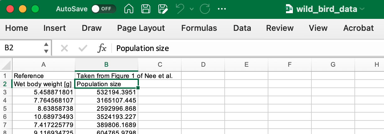
Sure enough the Excel file first row does contain additional information, a pointer to the article that this data was drawn from, and a quick Google reveals the article is [Nee, S., Read, A., Greenwood, J. et al. The relationship between abundance and body size in British birds. Nature 351, 312–313 (1991)] (https://www.nature.com/articles/351312a0)

Skipping a row

We could try to manually adjust things - remove the first row, change the column names, and then change the column types. But this is both a lot of work, and not really a best practice for data management. Lets instead re-read the data in with the skip option from read_excel, and see if it fixes all of our problems!

Code

wildbirds <- read_excel("_data/wild_bird_data.xlsx",
                        skip = 1)
wildbirds

This now looks great! Both variables are numeric, and now they correctly show up as double or (). The variable names might be a bit tough to work with, though, so it can be easier to assign new column names on the read in - and then manually adjust axis labels, etc once you are working on your publication-quality graphs.

Note that I skip two rows this time, and apply my own column names.

Code

wildbirds <- read_excel("_data/wild_bird_data.xlsx",
                        skip = 2, 
                        col_names = c("weight", "pop_size"))
wildbirds

Railroad (xls) ⭐⭐⭐⭐

The railroad data set is our most challenging data to read in this week, but is (by comparison) a fairly straightforward formatted table published by the Railroad Retirement Board. The value variable is a count of the number of employees in each county and state combination.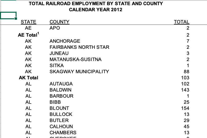

Looking at the excel file, we can see that there are only a few issues: 1. There are three rows at the top of the sheet that are not needed 2. There are blank columns that are not needed. 3. There are Total rows for each state that are not needed

Skipping title rows

For the first issue, we use the “skip” option on read_excel from the readxl package to skip the rows at the top.

Code

read_excel("_data/StateCounty2012.xls",
                     skip = 3)

New names:
• `` -> `...2`
• `` -> `...4`

Removing empty columns

For the second issue, I name the blank columns “delete” to make is easy to remove the unwanted columns. I then use select (with the ! sign to designate the complement or NOT) to select columns we wish to keep in the dataset - the rest are removed. Note that I skip 4 rows this time as I do not need the original header row.

There are other approaches you could use for this task (e.g., remove all columns that have no valid volues), but hard coding of variable names and types during data read in is not considered a violation of best practices and - if used strategically - can often make later data cleaning much easier.

Code

read_excel("_data/StateCounty2012.xls",
                     skip = 4,
                     col_names= c("State", "delete", "County", "delete", "Employees"))%>%
  select(!contains("delete"))

New names:
• `delete` -> `delete...2`
• `delete` -> `delete...4`

Filtering “total” rows

For the third issue, we are going to use filter to identify (and drop the rows that have the word “Total” in the State column). str_detect can be used to find specific rows within a column that have the designated “pattern”, while the “!” designates the complement of the selected rows (i.e., those without the “pattern” we are searching for.)

The str_detect command is from the stringr package, and is a powerful and easy to use implementation of grep and regex in the tidyverse - the base R functions (grep, gsub, etc) are classic but far more difficult to use, particularly for those not in practice. Be sure to explore the stringr package on your own.

Code

railroad<-read_excel("_data/StateCounty2012.xls",
                     skip = 4,
                     col_names= c("State", "delete", "County", "delete", "Employees"))%>%
  select(!contains("delete"))%>%
  filter(!str_detect(State, "Total"))

New names:
• `delete` -> `delete...2`
• `delete` -> `delete...4`

Code

railroad

Remove any table notes

Tables often have notes in the last few table rows. You can check table limits and use this information during data read-in to not read the notes by setting the n-max option at the total number of rows to read, or less commonly, the range option to specify the spreadsheet range in standard excel naming (e.g., “B4:R142”). If you didn’t handle this on read in, you can use the tail command to check for notes and either tail or head to keep only the rows that you need.

Code

tail(railroad, 10)

Code

#remove the last two observations
railroad <-head(railroad, -2)
tail(railroad, 10)

Confirm cases

And that is all it takes! The data are now ready for analysis. Lets see if we get the same number of unique states that were in the cleaned data in exercise 1.

Code

railroad%>%
  select(State)%>%
  n_distinct(.)

[1] 54

Code

railroad%>%
  select(State)%>%
  distinct()

Oh my goodness! It seems that we have an additional “State” - it looks like Canada is in the full excel data and not the tidy data. This is one example of why it is good practice to always work from the original data source!