library(tidyverse)
library(dplyr)
library(ggplot2)
library(readxl)

knitr::opts_chunk$set(echo = TRUE, warning=FALSE, message=FALSE)Final Project Assignment#2
final_Project_assignment_2
final_project_Exploratory_Analysis_and_Visualization
Exploratory Analysis and Visualization
Overview of the Final Project
Introduction:
Housing affordability is one of the major problems in the United States. With many households struggling to afford the rising cost of housing, it is critical to analyze the data trends over the country. According to statistics from the U.S. Census Bureau on median household income by city and region from 1996 to the present, Housing affordability has changed significantly over the time.
Although there has been general increase in median household income over the previous few decades, it has not been uniform across all the regions. Some regions have seen greater growth than others and similar swings have been observed in the median home prices, with some regions seeing more significant price increases than others.
The widening disparity between median household incomes and median property prices is one of the most obvious patterns in the statistics which is becoming more challenging for many Americans to afford homeownership as median property prices in many locations have been rising more quickly than median household incomes. The affordability issue has also been made worse by the fact that, despite the median household income rising, it has not kept up with the cost of living.
Overall, according to data from the U.S. Census Bureau, the affordability of housing has become a major worry over time, with many Americans finding it difficult to keep up with the rising cost of housing. The data emphasize the necessity of making policy changes to address the housing affordability crisis and guarantee that all Americans have access to safe, reasonably priced housing.
As part of this project I’m trying to focus on below: Visualize the trends in home values, the average household income, and inflation rates through time, broken down by area and city size. Create graphs showing the evolution of housing affordability over time in the country’s largest cities and how it differs by area and city size.
Data Sources:
As part of this project I found below resources that will help me understand the issue. Zillow Home Value Index (ZHVI) - a dataset from Zillow with the median home value for each region and city in the United States from 1996 to the present. https://www.kaggle.com/datasets/robikscube/zillow-home-value-index?resource=download
U.S. Census Bureau data on median household income by city and region from 1996 to the present. https://www.census.gov/data/tables/time-series/demo/income-poverty/historical-income-households.html
U.S. Bureau of Labor Statistics data on inflation rates by region and year from 1996 to the present. https://www.bls.gov/cpi/regional-resources.htm
- Util to Create a look up for states to region
state_to_region <- function(state) {
  region_lookup <- list(
    Northeast = c("Connecticut", "Maine", "Massachusetts", "New Hampshire", "New Jersey", "New York", "Pennsylvania", "Rhode Island", "Vermont"),
    South = c("Delaware", "District of Columbia", "Florida", "Georgia", "Maryland", "North Carolina", "South Carolina", "Virginia", "West Virginia", "Alabama", "Kentucky", "Mississippi", "Tennessee", "Arkansas", "Louisiana", "Oklahoma", "Texas"),
    Midwest = c("Illinois", "Indiana", "Michigan", "Ohio", "Wisconsin", "Iowa", "Kansas", "Minnesota", "Missouri", "Nebraska", "North Dakota", "South Dakota"),
    West = c("Arizona", "Colorado", "Idaho", "Montana", "Nevada", "New Mexico", "Utah", "Wyoming", "Alaska", "California", "Hawaii", "Oregon", "Washington")
  )
  region <- NA
  for (r in names(region_lookup)) {
    if (state %in% region_lookup[[r]]) {
      region <- r
      break
    }
  }
  return(region)
}- Read The Datasets
getwd()[1] "/Users/rahulsomu/Documents/DACSS_601/601_repo/posts"income_data <- read_excel("Rahul_Final_projectData/income_state.xlsx")
df_inflation <- read_excel("Rahul_Final_projectData/USA_inflation_data.xlsx")
df_rentalindex <- read.csv("Rahul_Final_projectData/ZHVI.csv")- Create functions for getting data for each state
#Function to get income data by state and year

get_median_se <- function(income_data, year, state){
  rownum <- which(income_data$State == state)
  colnum <- which(colnames(income_data) == year)
  median_income <- as.numeric(income_data[rownum, colnum])
  se <- as.numeric(income_data[rownum, colnum+1])
  #diff <- median_income - se
  return(c(as.character(median_income), as.character(se)))
}

get_median_se(income_data, "2021", "Alabama")
[1] "56929" "2294" #Function to get inflation data
avg_by_region_and_year <- function(df, state, year) {
region <- state_to_region(state)
subset_df <- subset(df, Region == region & Year == year)
row_avgs <- apply(subset_df[, 4:ncol(subset_df)], 1, mean, na.rm = TRUE)
overall_avg <- mean(row_avgs, na.rm = TRUE)
return(overall_avg)
}
# example usage
avg_by_region_and_year(df_inflation, "Texas", 2000)[1] 167.4143df_rentalindex$Date <- as.Date(df_rentalindex$Date, format = "%Y-%m-%d")
# function to calculate average rental index for a state and year
get_state_rentalindex <- function(df,state, year) {
df_filtered <- subset(df, format(as.Date(Date), "%Y") == year)
state_new <- chartr(" ", ".", state)
state_avg <- mean(df_filtered[[state_new]])
return(state_avg)
}
# example usage
get_state_rentalindex(df_rentalindex,"District of Columbia", "2000")[1] 153953.9- present the descriptive information of the dataset(s) using the functions in Challenges 1, 2, and 3;
dim(income_data)[1] 53 79dim(df_inflation)[1] 96 17dim(df_rentalindex)[1] 278 52head(income_data)- conduct summary statistics of the dataset(s); especially show the basic statistics (min, max, mean, median, etc.) for the variables you are interested in.
summary(df_rentalindex) Date Virginia California Florida
Min. :2000-01-01 Min. :114448 Min. :183263 Min. :102232
1st Qu.:2005-10-08 1st Qu.:197891 1st Qu.:292524 1st Qu.:136109
Median :2011-07-16 Median :219631 Median :388784 Median :173778
Mean :2011-07-17 Mean :219795 Mean :400685 Mean :188378
3rd Qu.:2017-04-23 3rd Qu.:245837 3rd Qu.:471709 3rd Qu.:230129
Max. :2023-02-01 Max. :352788 Max. :758837 Max. :382968
Texas Nevada New.York New.Jersey
Min. :103491 Min. :126840 Min. :122871 Min. :151148
1st Qu.:123530 1st Qu.:167170 1st Qu.:204061 1st Qu.:247960
Median :130655 Median :220389 Median :219991 Median :279515
Mean :151983 Mean :237218 Mean :232584 Mean :281958
3rd Qu.:177563 3rd Qu.:303531 3rd Qu.:253952 3rd Qu.:317507
Max. :295310 Max. :440144 Max. :410896 Max. :440368
Arizona Tennessee West.Virginia Georgia
Min. :127957 Min. : 92784 Min. : 58201 Min. :106693
1st Qu.:151352 1st Qu.:111305 1st Qu.: 78830 1st Qu.:126001
Median :189184 Median :120526 Median : 83142 Median :140309
Mean :209957 Mean :137849 Mean : 88792 Mean :153769
3rd Qu.:252451 3rd Qu.:150538 3rd Qu.:100596 3rd Qu.:159109
Max. :437047 Max. :285261 Max. :143983 Max. :303796
North.Carolina Massachusetts Hawaii Colorado
Min. :116314 Min. :183093 Min. :176017 Min. :169818
1st Qu.:135109 1st Qu.:285744 1st Qu.:369539 1st Qu.:214326
Median :145608 Median :317222 Median :419144 Median :228125
Mean :159663 Mean :333554 Mean :438470 Mean :278369
3rd Qu.:165305 3rd Qu.:369005 3rd Qu.:554296 3rd Qu.:339056
Max. :303166 Max. :557412 Max. :861627 Max. :556750
Michigan South.Carolina Vermont Minnesota
Min. : 79031 Min. :100082 Min. : 88760 Min. :112685
1st Qu.:100723 1st Qu.:122438 1st Qu.:150899 1st Qu.:156275
Median :116302 Median :134929 Median :168068 Median :177589
Mean :121370 Mean :145298 Mean :174899 Mean :186909
3rd Qu.:127914 3rd Qu.:154536 3rd Qu.:197476 3rd Qu.:205064
Max. :211833 Max. :267835 Max. :319746 Max. :314021
Indiana Washington Illinois Oregon
Min. : 90242 Min. :166298 Min. :108150 Min. :142976
1st Qu.:103664 1st Qu.:216225 1st Qu.:132659 1st Qu.:188999
Median :109106 Median :259786 Median :150891 Median :229912
Mean :121298 Mean :289661 Mean :154393 Mean :254140
3rd Qu.:127750 3rd Qu.:326684 3rd Qu.:173109 3rd Qu.:306743
Max. :217822 Max. :588018 Max. :229898 Max. :498337
Connecticut Utah North.Dakota Montana
Min. :156392 Min. :161827 Min. :130966 Min. :144789
1st Qu.:227901 1st Qu.:178131 1st Qu.:131628 1st Qu.:166461
Median :246940 Median :212460 Median :133798 Median :174723
Mean :248507 Mean :245073 Mean :159585 Mean :205339
3rd Qu.:272082 3rd Qu.:274825 3rd Qu.:192546 3rd Qu.:222790
Max. :349739 Max. :529454 Max. :235975 Max. :434557
New.Hampshire Ohio Missouri Maryland
Min. :125228 Min. : 94815 Min. : 84986 Min. :138999
1st Qu.:197957 1st Qu.:104970 1st Qu.:108511 1st Qu.:223950
Median :219170 Median :112999 Median :118146 Median :255487
Mean :232154 Mean :120513 Mean :126813 Mean :255882
3rd Qu.:245854 3rd Qu.:123063 3rd Qu.:134601 3rd Qu.:296146
Max. :421924 Max. :199518 Max. :221340 Max. :381710
Idaho Wisconsin Kansas Pennsylvania
Min. :115460 Min. :102168 Min. : 72593 Min. : 87544
1st Qu.:136513 1st Qu.:128707 1st Qu.: 92599 1st Qu.:135443
Median :170597 Median :142384 Median : 98660 Median :143779
Mean :197345 Mean :150836 Mean :109496 Mean :146101
3rd Qu.:210504 3rd Qu.:158847 3rd Qu.:120684 3rd Qu.:154896
Max. :470980 Max. :250226 Max. :205073 Max. :237774
Oklahoma District.of.Columbia Nebraska Alaska
Min. : 70112 Min. :147817 Min. : 99521 Min. :125485
1st Qu.: 87542 1st Qu.:326460 1st Qu.:115634 1st Qu.:200767
Median : 94748 Median :358798 Median :120794 Median :229993
Mean :103287 Mean :389287 Mean :135590 Mean :232676
3rd Qu.:112466 3rd Qu.:501651 3rd Qu.:148736 3rd Qu.:263890
Max. :185171 Max. :654749 Max. :236836 Max. :343188
New.Mexico Wyoming Delaware Rhode.Island
Min. :123686 Min. :130764 Min. :132902 Min. :125136
1st Qu.:149589 1st Qu.:161553 1st Qu.:193728 1st Qu.:209214
Median :161310 Median :188812 Median :220943 Median :234743
Mean :166271 Mean :195671 Mean :221938 Mean :243631
3rd Qu.:176335 3rd Qu.:220578 3rd Qu.:247511 3rd Qu.:278837
Max. :277310 Max. :319529 Max. :351269 Max. :404953
Maine Louisiana Arkansas Alabama
Min. : 92612 Min. : 83285 Min. : 69180 Min. : 76906
1st Qu.:153086 1st Qu.:110090 1st Qu.: 91542 1st Qu.: 91983
Median :166698 Median :124074 Median : 97689 Median :103500
Mean :177752 Mean :126170 Mean :103042 Mean :111666
3rd Qu.:189259 3rd Qu.:140977 3rd Qu.:113094 3rd Qu.:122263
Max. :344147 Max. :180360 Max. :173423 Max. :199357
Mississippi South.Dakota Iowa Kentucky
Min. : 66101 Min. : 90148 Min. : 75996 Min. : 78366
1st Qu.: 83544 1st Qu.:114397 1st Qu.: 97729 1st Qu.: 96390
Median : 88905 Median :124808 Median :101922 Median :101124
Mean : 96463 Mean :144178 Mean :113321 Mean :109261
3rd Qu.:111732 3rd Qu.:169210 3rd Qu.:126571 3rd Qu.:116845
Max. :156641 Max. :275894 Max. :194074 Max. :184542 Combining all the dataframes to a single dataframe
# Create an empty data frame to store the results
result_df <- data.frame(State = character(),
                        Year = character(),
                        Median_Income = numeric(),
                        Standard_Error = numeric(),
                        Inflation_Average = numeric(),
                        Rental_Index = numeric(),
                        stringsAsFactors = FALSE)

# Loop through each state and year
for (state in unique(income_data$State)) {
  for (year in 2000:2020) {
    median_se <- get_median_se(income_data, as.character(year),as.character(state))
    inflation_avg <- avg_by_region_and_year(df_inflation, as.character(state), as.character(year))
    rental_index <- get_state_rentalindex(df_rentalindex, as.character(state), as.character(year))
    #print(median_se,inflation_avg,rental_index)
    # Add the calculated values to the result data frame
    result_df <- rbind(result_df, data.frame(State = state,
                                             Year = as.character(year),
                                             Median_Income = as.numeric(median_se[1]),
                                             Standard_Error = as.numeric(median_se[2]),
                                             Inflation_Average = inflation_avg,
                                             Rental_Index = rental_index,
                                             stringsAsFactors = FALSE))
  }
}

# Print the resulting data frame
result_df <- result_df %>%
  filter(!is.na(State) & State != "United States")

library(ggplot2)

# Calculate the affordability score
result_df$Affordability_Score <- result_df$Rental_Index / result_df$Median_Income * (1 + result_df$Inflation_Average)

# Categorize states based on affordability score
# Categorize states based on affordability score range
result_df$Affordability_Category <- cut(result_df$Affordability_Score,
                                        breaks = c(-Inf, 1000, 1500, Inf),
                                        labels = c("Unaffordable", "Moderately Affordable", "Affordable"),
                                        include.lowest = TRUE)


result_df- Heatmap of Affordability Scores: The heatmap, also known as a “heatmap” in the code, shows the evolution of a state’s affordability score over time. Each heatmap cell represents a state and a certain year, while the fill color represents the affordability category. Green is used to indicate “Affordable,” yellow to indicate “Moderately Affordable,” and red to indicate “Unaffordable.”
We can see how affordability categories have changed over time, across states and years, thanks to the heatmap. It makes it easier to spot states that consistently fall into a particular affordability group as well as those where affordability changes over time. Policymakers and academics can easily identify states that need attention in terms of housing affordability by displaying the data in this way and can then prioritize measures accordingly.
- Median Real Incomes Over Time: The median real incomes over time for each state are shown in a line plot (referred to as “income_plot” in the code). Each line displays the median real income trend for a particular state, with the years on the x-axis and the median income on the y-axis.
With the help of this image, we can see how the median real income has changed among states and spot any trends or inequalities. It offers insights into the economic health of various states and aids in understanding how median wages have changed over time. This visualization can be used by researchers and policymakers to examine probable causes of income inequality, identify states with large changes in median earnings, and evaluate patterns in income growth.
# Heatmap of affordability scores
heatmap <- ggplot(result_df, aes(x = Year, y = State, fill = Affordability_Category)) +
  geom_tile() +
  scale_fill_manual(values = c("Affordable" = "green", "Moderately Affordable" = "yellow", "Unaffordable" = "red")) +
  labs(x = "Year", y = "State", fill = "Affordability Category") +
  theme_classic()
# Display the visualizations
heatmap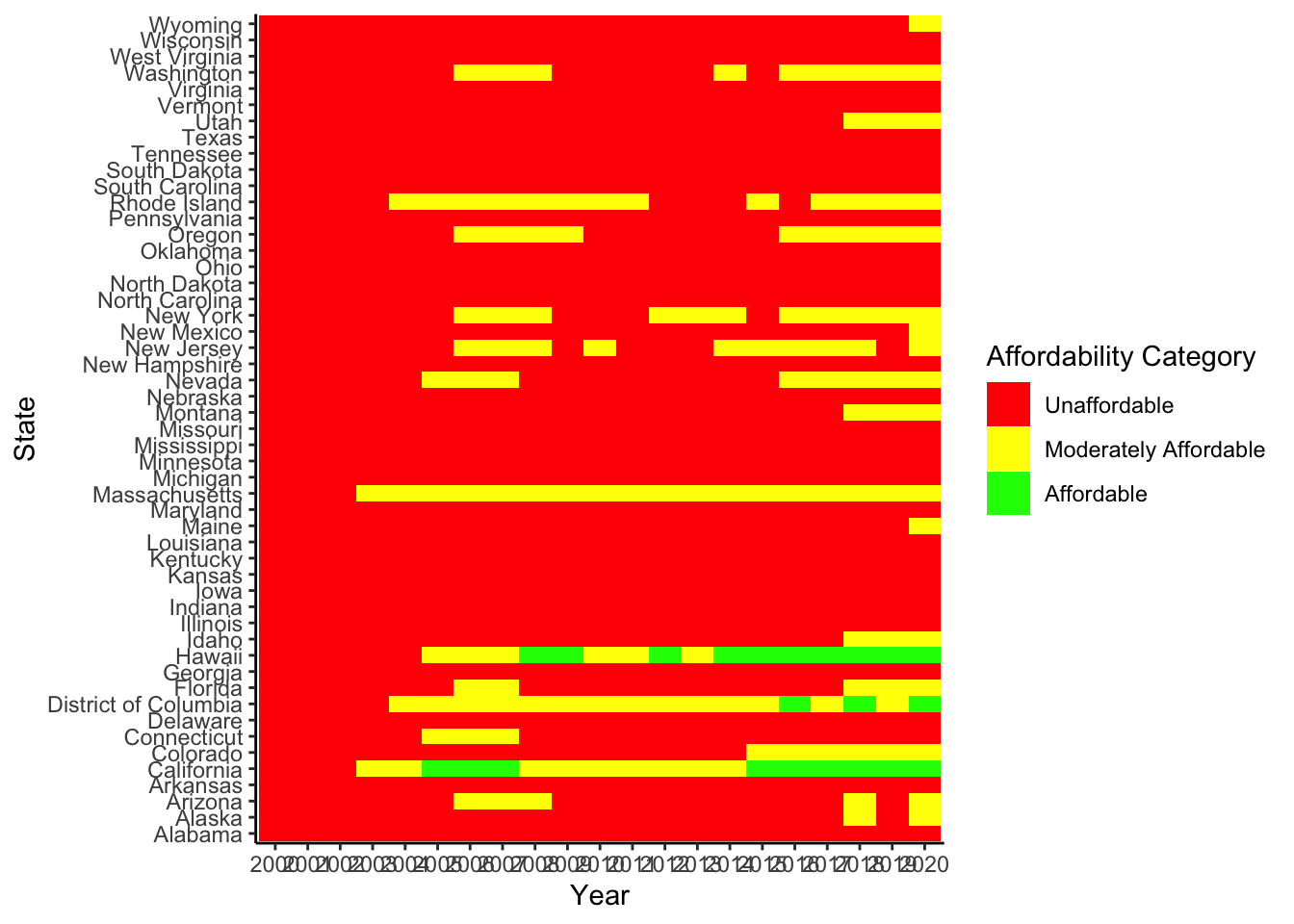
- Median Real Incomes Over Time: The median real incomes over time for each state are shown in a line plot (referred to as “income_plot” in the code). Each line displays the median real income trend for a particular state, with the years on the x-axis and the median income on the y-axis.
With the help of this image, we can see how the median real income has changed among states and spot any trends or inequalities. It offers insights into the economic health of various states and aids in understanding how median wages have changed over time. This visualization can be used by researchers and policymakers to examine probable causes of income inequality, identify states with large changes in median earnings, and evaluate patterns in income growth.
# Plot median real incomes over time
income_plot <- ggplot(result_df, aes(x = Year, y = Median_Income, group = State)) +
  geom_line() +
  labs(x = "Year", y = "Median Income", title = "Median Real Incomes Over Time") +
  theme_bw()


income_plot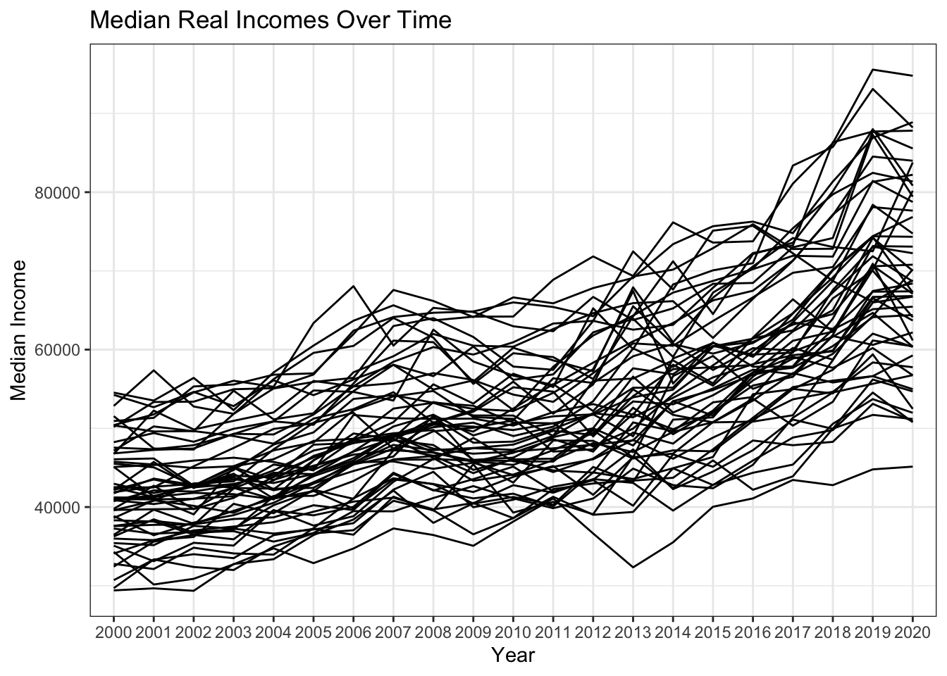
Median Income by Year: Plot 1 depicts the median income trend for all states throughout time. It enables us to track changes in median income over time and get knowledge of state-by-state income growth trends.
library(ggplot2)

plot1 <- ggplot(result_df, aes(x = Year, y = Median_Income, color = State)) +
  geom_point() +
  labs(x = "Year", y = "Median Income", title = "Median Income by Year") +
  theme_bw()

# Adjust the size of the points if needed
plot1 + geom_point(size = 3)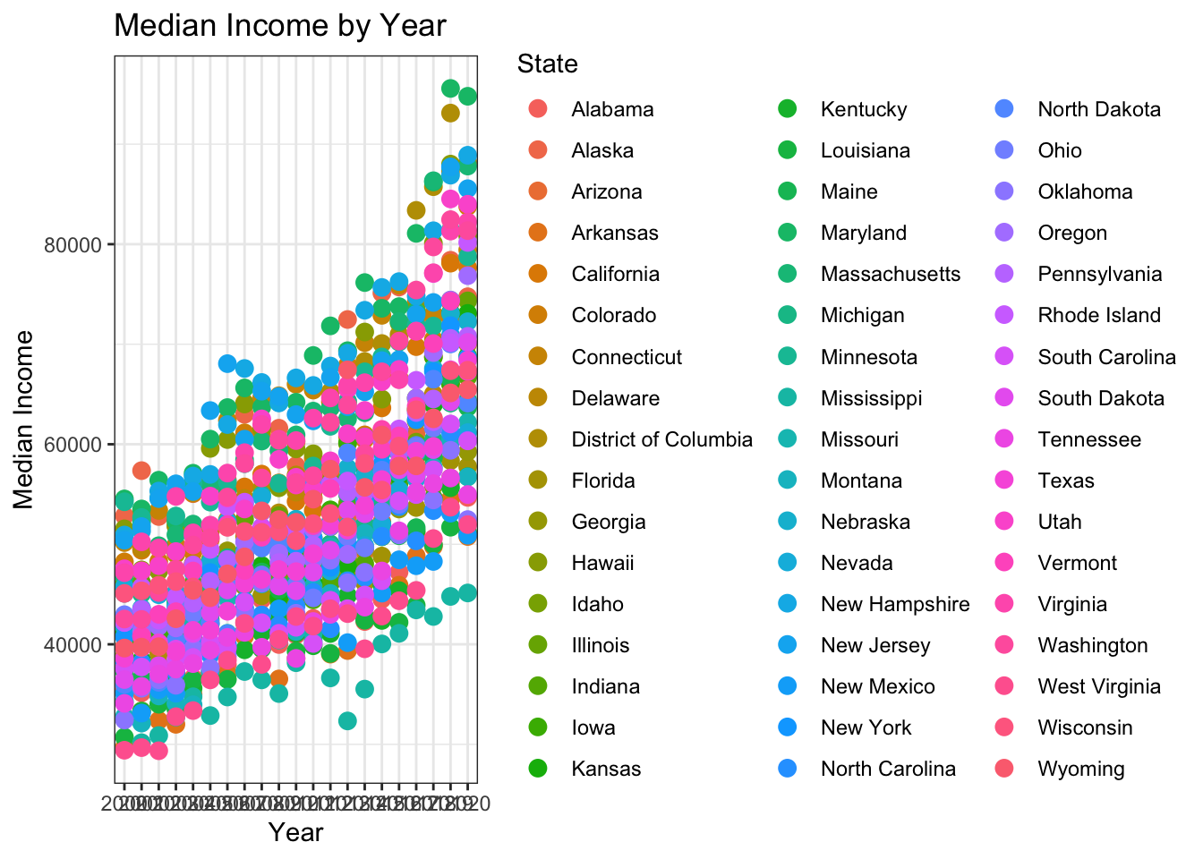
Rental Index by State: Plot 2 displays a box plot that shows how the rental index values are distributed among the states. It aids in comprehending price fluctuation and locating possible outliers or states with higher or lower rental rates.
plot2 <- ggplot(result_df, aes(x = State, y = Rental_Index)) +
  geom_boxplot() +
  labs(x = "State", y = "Rental Index", title = "Rental Index by State") +
  theme_bw()

plot2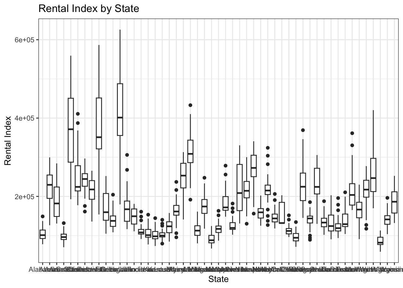
Distribution of Affordability Categories: Plot 3 shows how States are distributed across Affordability Categories. It gives a general summary of how many states fall into each of the three affordability categories—“Affordable,” “Moderately Affordable,” and “Unaffordable.” This image makes it possible to quickly evaluate the affordability environment as a whole.
plot3 <- ggplot(result_df, aes(x = Affordability_Category, fill = Affordability_Category)) +
  geom_bar() +
  labs(x = "Affordability Category", y = "Count", title = "Affordability Category Distribution") +
  theme_bw()

plot3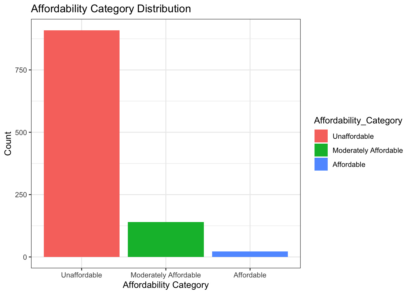
Average inflation versus median income: Plot 4 shows a scatter plot of the median income versus the average inflation rate, with each point denoting a different state. This map makes it easier to spot any possible connections or correlations between state-by-state inflation rates and income levels.
plot4 <- ggplot(result_df, aes(x = Median_Income, y = Inflation_Average, color = State)) +
  geom_point() +
  labs(x = "Median Income", y = "Inflation Average", title = "Median Income vs. Inflation Average") +
  theme_bw()

plot4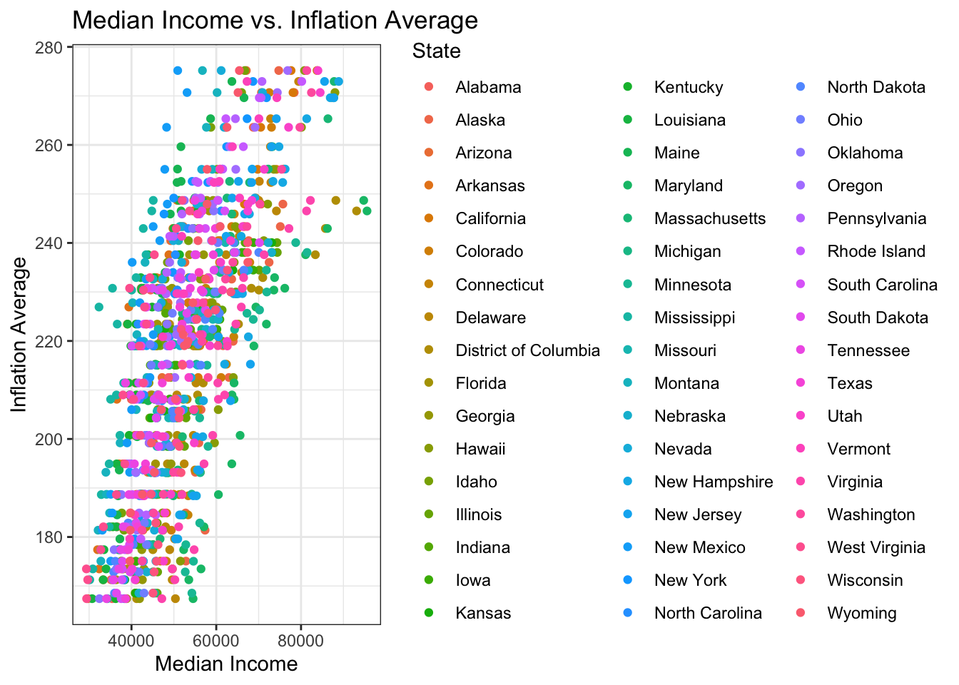
Plot 6 displays a bar chart comparing the number of states in each affordability category across various states. It allows us to track the regional distribution of the affordability categories and pinpoint which states have more or lower representation in each one.
plot6 <- ggplot(result_df, aes(x = State, fill = Affordability_Category)) +
  geom_bar() +
  labs(x = "State", y = "Count", title = "Affordability Category by State") +
  theme_bw() +
  theme(axis.text.x = element_text(angle = 45, hjust = 1))

plot6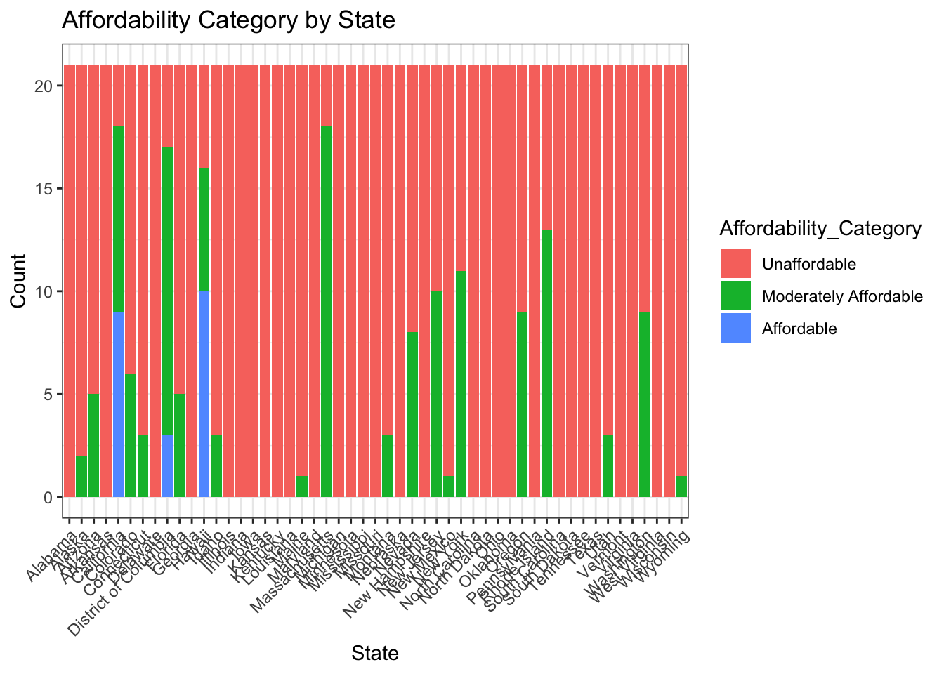
Rental Index by Affordability Category: Plot 7 makes use of a violin plot to show how the rental index values are distributed among different affordability groups. With an awareness of the rental market within each affordability category, this graphic offers insights on the relationship between affordability and rental costs.
plot7 <- ggplot(result_df, aes(x = Affordability_Category, y = Rental_Index)) +
  geom_violin() +
  labs(x = "Affordability Category", y = "Rental Index", title = "Rental Index by Affordability Category") +
  theme_bw()

plot7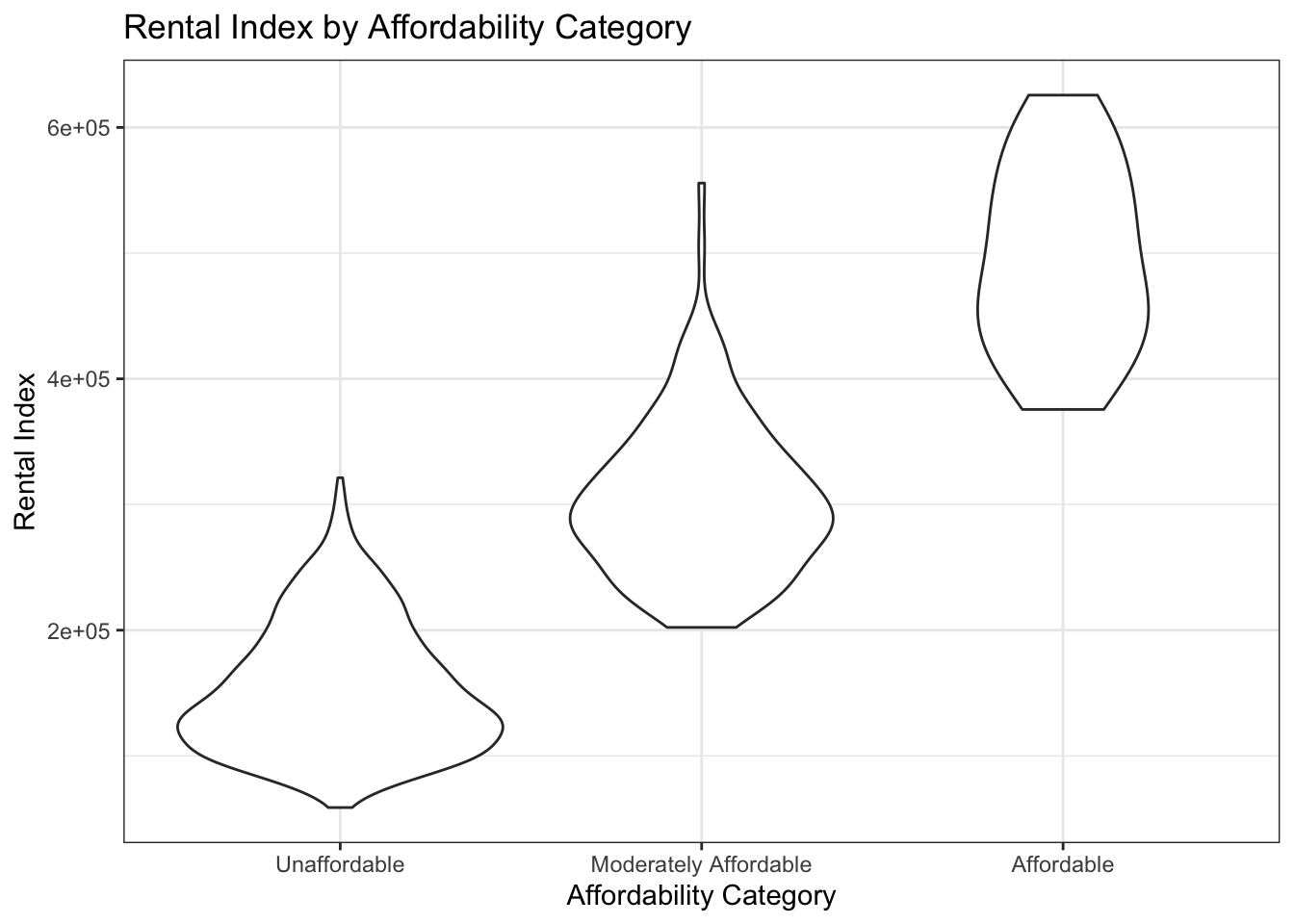
State-by-State Median Income: Plot 8 displays a bar graph showing the median income for each state. It makes it simple to compare income levels between states, making it easier to determine which states have higher or lower median incomes.
plot8 <- ggplot(result_df, aes(x = State, y = Median_Income, fill = State)) +
  geom_bar(stat = "identity") +
  labs(x = "State", y = "Median Income", title = "Median Income by State") +
  theme_bw() +
  theme(axis.text.x = element_text(angle = 45, hjust = 1))

plot8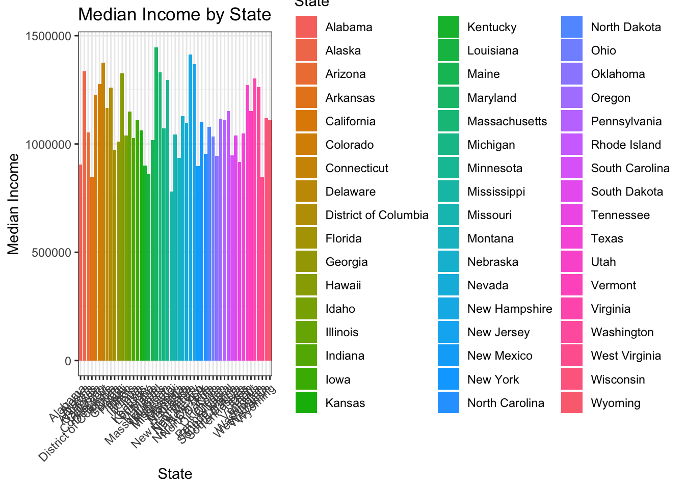
Inflation Average by Year Plotted as a Bar Graph: The bar graph shows the inflation average by year, with each bar representing a different year. Each bar’s height shows the average inflation rate, while the fill color denotes various states.
plot9 <- ggplot(result_df, aes(x = Year, y = Inflation_Average, fill = State)) +
  geom_bar(stat = "identity", position = "dodge") +
  labs(x = "Year", y = "Inflation Average", title = "Inflation Average by Year") +
  theme_bw()

plot9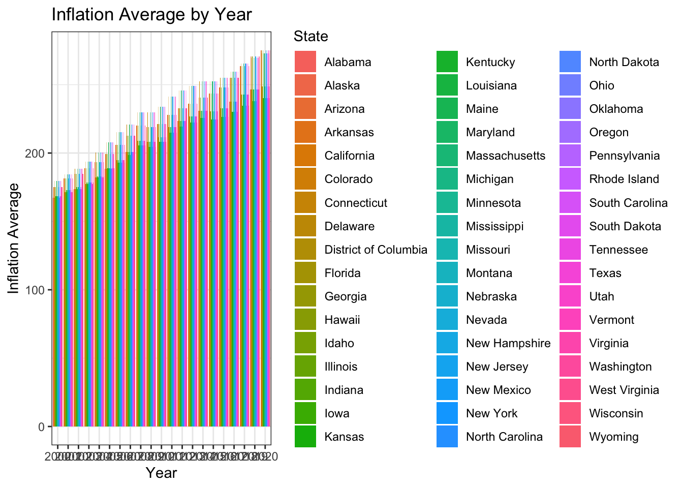
The analysis of housing affordability trends utilizing information on median household income, inflation rates, and rental indices has, in conclusion, shown the complex housing affordability situation in the United States. The results emphasize the growing gap between median salaries and housing prices, which makes it more challenging for many Americans to finance homeownership.
We have learned a lot about how housing affordability has changed over time, how it differs between states, and how income, inflation, and rental costs are related by utilizing visualizations like heatmaps, line graphs, box plots, scatter plots, and bar charts. Policymakers, researchers, and other stakeholders can use these visualizations to better understand the dynamics of housing affordability and to help them decide how to handle the housing problem.
Significant differences in housing affordability between states have been found by the investigation, with most of states constantly falling into the “Unaffordable” category. This emphasizes the requirement for focused governmental interventions and actions to tackle affordability issues and guarantee that all Americans have access to safe and reasonably priced housing.
The visualizations have also demonstrated how economic factors like inflation affect housing affordability. In order to devise methods to lessen the impact of growing expenses on household budgets, it can be helpful to understand the relationship between the median income and inflation rates.
The report as a whole emphasizes how urgent it is to address the housing affordability situation in the US. It is possible to work toward a future where affordable housing is available to everyone by utilizing data-driven insights and enacting tailored policies, allowing individuals and families to prosper and contribute to vibrant and sustainable communities.