library(tidyverse)
library(dplyr)
library(ggplot2)
library(readxl)

knitr::opts_chunk$set(echo = TRUE, warning=FALSE, message=FALSE)Final Project: Complete Write-up
final_Project
final_project_complete_writeup
Analyzing Housing Market Trends, Income Levels, and Inflation: A Comprehensive Study
Overview of the Final Project
Introduction:
Housing affordability is one of the major problems in the United States. With many households struggling to afford the rising cost of housing, it is critical to analyze the data trends over the country. According to statistics from the U.S. Census Bureau on median household income by city and region from 1996 to the present, Housing affordability has changed significantly over the time.
Although there has been general increase in median household income over the previous few decades, it has not been uniform across all the regions. Some regions have seen greater growth than others and similar swings have been observed in the median home prices, with some regions seeing more significant price increases than others.
The widening disparity between median household incomes and median property prices is one of the most obvious patterns in the statistics which is becoming more challenging for many Americans to afford homeownership as median property prices in many locations have been rising more quickly than median household incomes. The affordability issue has also been made worse by the fact that, despite the median household income rising, it has not kept up with the cost of living.
Overall, according to data from the U.S. Census Bureau, the affordability of housing has become a major worry over time, with many Americans finding it difficult to keep up with the rising cost of housing. The data emphasize the necessity of making policy changes to address the housing affordability crisis and guarantee that all Americans have access to safe, reasonably priced housing.
As part of this project I’m trying to focus on below: Visualize the trends in home values, the average household income, and inflation rates through time, broken down by area and city size. Create graphs showing the evolution of housing affordability over time in the country’s largest cities and how it differs by area and city size.
Data Sources and description:
1.Zillow Home Value Index (ZHVI) Dataset: As part of this project I found a dataset that will help me understand the issue. Zillow Home Value Index (ZHVI) - a dataset from Zillow with the median home value for each region and city in the United States from 1996 to the present.
The ZHVI dataset provides a comprehensive information on home values all over the United States.This dataset helps gain insights in the housing market to . Key metrics to consider include median home values, year-over-year changes, and regional variations. These numbers will help us understand the fluctuations in housing prices and identify areas experiencing rapid growth or decline.
Historical Income by Households Dataset:
U.S. Census Bureau provides information on income levels over time which helps us Analyse and track changes in household incomes, including median income, income distribution, and income inequality. With these numbers, we can assess the purchasing power of individuals and the affordability of housing in relation to income levels.
Regional Consumer Price Index (CPI) Dataset:
The Regional CPI dataset from the BLS provides data on inflation rates across United States helps us with the information to Analyse this dataset and enables us to understand how inflation impacts housing prices and overall cost of living. By examining regional inflation rates alongside housing market trends, we can identify how housing affordability may be affected by inflationary pressures.
https://www.kaggle.com/datasets/robikscube/zillow-home-value-index?resource=download
U.S. Census Bureau data on median household income by city and region from 1996 to the present. https://www.census.gov/data/tables/time-series/demo/income-poverty/historical-income-households.html
U.S. Bureau of Labor Statistics data on inflation rates by region and year from 1996 to the present. https://www.bls.gov/cpi/regional-resources.htm
Below we create some utils and combine them to a single dataframe: Util to Create a look up for states to region
state_to_region <- function(state) {
  region_lookup <- list(
    Northeast = c("Connecticut", "Maine", "Massachusetts", "New Hampshire", "New Jersey", "New York", "Pennsylvania", "Rhode Island", "Vermont"),
    South = c("Delaware", "District of Columbia", "Florida", "Georgia", "Maryland", "North Carolina", "South Carolina", "Virginia", "West Virginia", "Alabama", "Kentucky", "Mississippi", "Tennessee", "Arkansas", "Louisiana", "Oklahoma", "Texas"),
    Midwest = c("Illinois", "Indiana", "Michigan", "Ohio", "Wisconsin", "Iowa", "Kansas", "Minnesota", "Missouri", "Nebraska", "North Dakota", "South Dakota"),
    West = c("Arizona", "Colorado", "Idaho", "Montana", "Nevada", "New Mexico", "Utah", "Wyoming", "Alaska", "California", "Hawaii", "Oregon", "Washington")
  )
  region <- NA
  for (r in names(region_lookup)) {
    if (state %in% region_lookup[[r]]) {
      region <- r
      break
    }
  }
  return(region)
}
Read The Datasets
getwd()[1] "/Users/rahulsomu/Documents/DACSS_601/601_repo/posts"income_data <- read_excel("Rahul_Final_projectData/income_state.xlsx")
df_inflation <- read_excel("Rahul_Final_projectData/USA_inflation_data.xlsx")
df_rentalindex <- read.csv("Rahul_Final_projectData/ZHVI.csv")Create functions for getting data for each state
#Function to get income data by state and year

get_median_se <- function(income_data, year, state){
  rownum <- which(income_data$State == state)
  colnum <- which(colnames(income_data) == year)
  median_income <- as.numeric(income_data[rownum, colnum])
  se <- as.numeric(income_data[rownum, colnum+1])
  #diff <- median_income - se
  return(c(as.character(median_income), as.character(se)))
}

get_median_se(income_data, "2021", "Alabama")
[1] "56929" "2294" #Function to get inflation data
avg_by_region_and_year <- function(df, state, year) {
region <- state_to_region(state)
subset_df <- subset(df, Region == region & Year == year)
row_avgs <- apply(subset_df[, 4:ncol(subset_df)], 1, mean, na.rm = TRUE)
overall_avg <- mean(row_avgs, na.rm = TRUE)
return(overall_avg)
}
# example usage
avg_by_region_and_year(df_inflation, "Texas", 2000)[1] 167.4143df_rentalindex$Date <- as.Date(df_rentalindex$Date, format = "%Y-%m-%d")
# function to calculate average rental index for a state and year
get_state_rentalindex <- function(df,state, year) {
df_filtered <- subset(df, format(as.Date(Date), "%Y") == year)
state_new <- chartr(" ", ".", state)
state_avg <- mean(df_filtered[[state_new]])
return(state_avg)
}
# example usage
get_state_rentalindex(df_rentalindex,"District of Columbia", "2000")[1] 153953.9Combining all the dataframes to a single dataframe
# Create an empty data frame to store the results
result_df <- data.frame(State = character(),
                        Year = character(),
                        Median_Income = numeric(),
                        Standard_Error = numeric(),
                        Inflation_Average = numeric(),
                        Rental_Index = numeric(),
                        stringsAsFactors = FALSE)

# Loop through each state and year
for (state in unique(income_data$State)) {
  for (year in 2000:2020) {
    median_se <- get_median_se(income_data, as.character(year),as.character(state))
    inflation_avg <- avg_by_region_and_year(df_inflation, as.character(state), as.character(year))
    rental_index <- get_state_rentalindex(df_rentalindex, as.character(state), as.character(year))
    #print(median_se,inflation_avg,rental_index)
    # Add the calculated values to the result data frame
    result_df <- rbind(result_df, data.frame(State = state,
                                             Year = as.character(year),
                                             Median_Income = as.numeric(median_se[1]),
                                             Standard_Error = as.numeric(median_se[2]),
                                             Inflation_Average = inflation_avg,
                                             Rental_Index = rental_index,
                                             stringsAsFactors = FALSE))
  }
}

# Print the resulting data frame
result_df <- result_df %>%
  filter(!is.na(State) & State != "United States")

library(ggplot2)

# Calculate the affordability score
result_df$Affordability_Score <- result_df$Rental_Index / result_df$Median_Income * (1 + result_df$Inflation_Average)

# Categorize states based on affordability score
# Categorize states based on affordability score range
result_df$Affordability_Category <- cut(result_df$Affordability_Score,
                                        breaks = c(-Inf, 1000, 1500, Inf),
                                        labels = c("Unaffordable", "Moderately Affordable", "Affordable"),
                                        include.lowest = TRUE)


result_df
Dataset Description: The combined dataset consists of 1071 rows with 8 columnns named “State”,“Year”,“Median_Income”,“Standard_Error”,“Inflation_Average”,“Rental_Index”,“Affordability_Score”,“Affordability_Category” with information for last two decades.
dim(result_df)[1] 1071 8colnames(result_df)[1] "State" "Year" "Median_Income"
[4] "Standard_Error" "Inflation_Average" "Rental_Index"
[7] "Affordability_Score" "Affordability_Category"##Analysis Plan: To categorize the states, a composite index that takes into account of major factors as Zillow Home Value Index (ZHVI) , median household income by state, inflation rates by region.Index on healthy housing affordability could be done using below formula: Affordability Score = (ZHVI / Income) * (1 + Inflation) Variables: Zillow Home Value Index (ZHVI) - Measure of median home value in each state, Median household income by state - average income earned by households in each state, Inflation rates by region - Measure of change in prices of goods and services over time in each region.
To visualize the affordability, based on affordabilty score the states are divided into three categories : “Affordable”, “Moderately Affordable”, and “Unaffordable”.
Affordable: States with a score above 1500, indicating that housing is relatively affordable compared to income levels. Moderately Affordable: States with a score between 1000 and 1500, indicating that housing is somewhat affordable but may be becoming less so over time. Unaffordable: States with a score above 1000, indicating that housing is significantly unaffordable relative to income levels and inflation rates.
With CPI prices for the states available between 2000 and 2023 and then compare median real incomes in these cities for the respective periods. First, we convert 2011 median incomes grouped by the city into 2018 dollars by using CPI’s of both time periods.
Based on the categories, Let’s make some visualisations to help us understand the visualisations.
- Heatmap of Affordability Scores: The heatmap, also known as a “heatmap” in the code, shows the evolution of a state’s affordability score over time. Each heatmap cell represents a state and a certain year, while the fill color represents the affordability category. Green is used to indicate “Affordable,” yellow to indicate “Moderately Affordable,” and red to indicate “Unaffordable.”
We can see how affordability categories have changed over time, across states and years, thanks to the heatmap. It makes it easier to spot states that consistently fall into a particular affordability group as well as those where affordability changes over time. Policymakers and academics can easily identify states that need attention in terms of housing affordability by displaying the data in this way and can then prioritize measures accordingly.
# Heatmap of affordability scores
heatmap <- ggplot(result_df, aes(x = Year, y = State, fill = Affordability_Category)) +
  geom_tile() +
  scale_fill_manual(values = c("Affordable" = "green", "Moderately Affordable" = "yellow", "Unaffordable" = "red")) +
  labs(x = "Year", y = "State", fill = "Affordability Category") +
  theme_classic()
# Display the visualizations
heatmap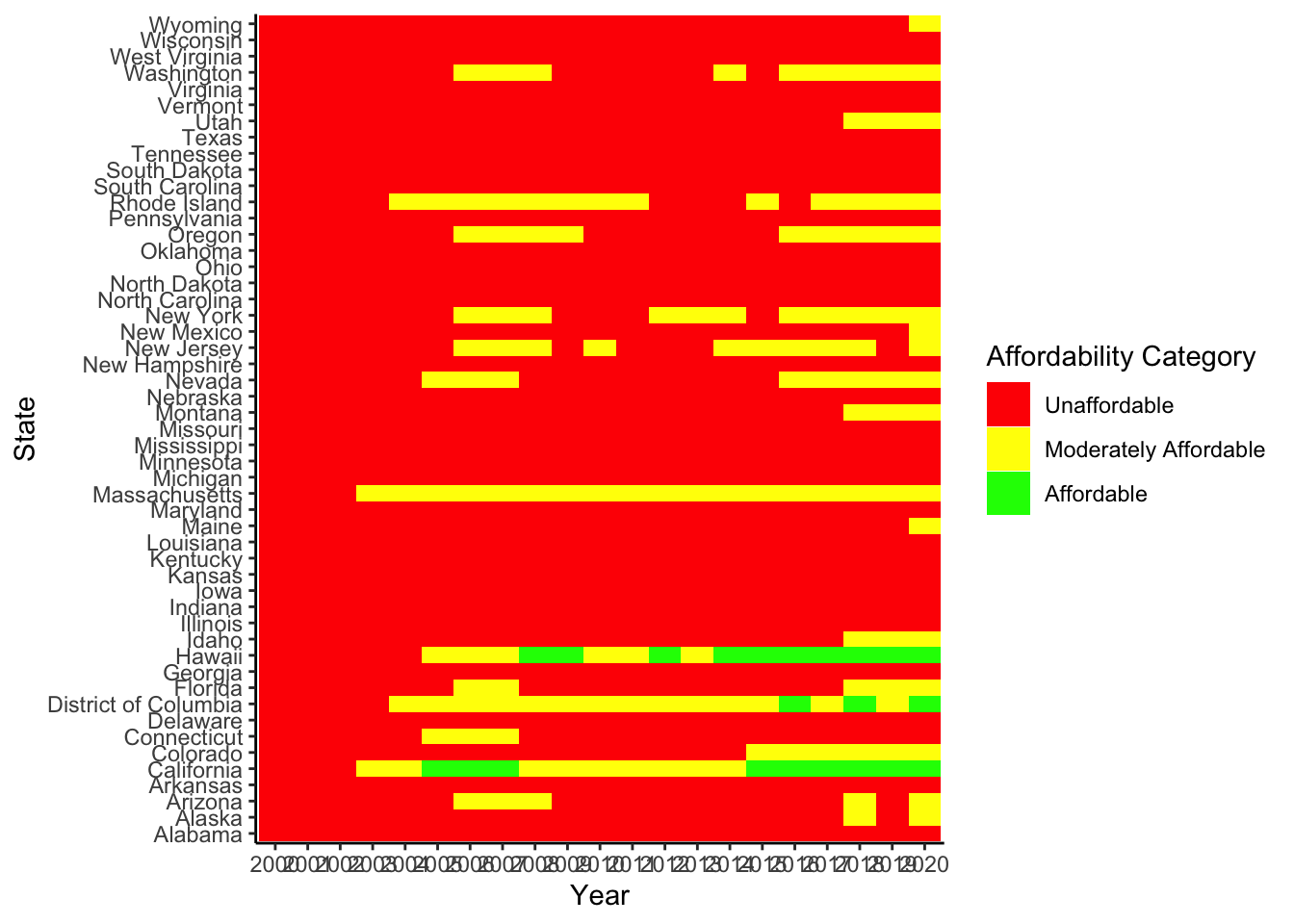
- Median Real Incomes Over Time: The median real incomes over time for each state are shown in a line plot (referred to as “income_plot” in the code). Each line displays the median real income trend for a particular state, with the years on the x-axis and the median income on the y-axis.
With the help of this image, we can see how the median real income has changed among states and spot any trends or inequalities. It offers insights into the economic health of various states and aids in understanding how median wages have changed over time. This visualization can be used by researchers and policymakers to examine probable causes of income inequality, identify states with large changes in median earnings, and evaluate patterns in income growth.
# Plot median real incomes over time
income_plot <- ggplot(result_df, aes(x = Year, y = Median_Income, group = State)) +
  geom_line() +
  labs(x = "Year", y = "Median Income", title = "Median Real Incomes Over Time") +
  theme_bw()


income_plot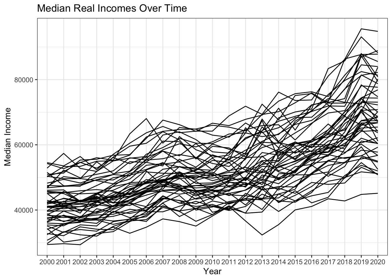
Median Income by Year: Plot 1 depicts the median income trend for all states throughout time. It enables us to track changes in median income over time and get knowledge of state-by-state income growth trends.
library(ggplot2)

plot1 <- ggplot(result_df, aes(x = Year, y = Median_Income, color = State)) +
  geom_point() +
  labs(x = "Year", y = "Median Income", title = "Median Income by Year") +
  theme_bw()

# Adjust the size of the points if needed
plot1 + geom_point(size = 3)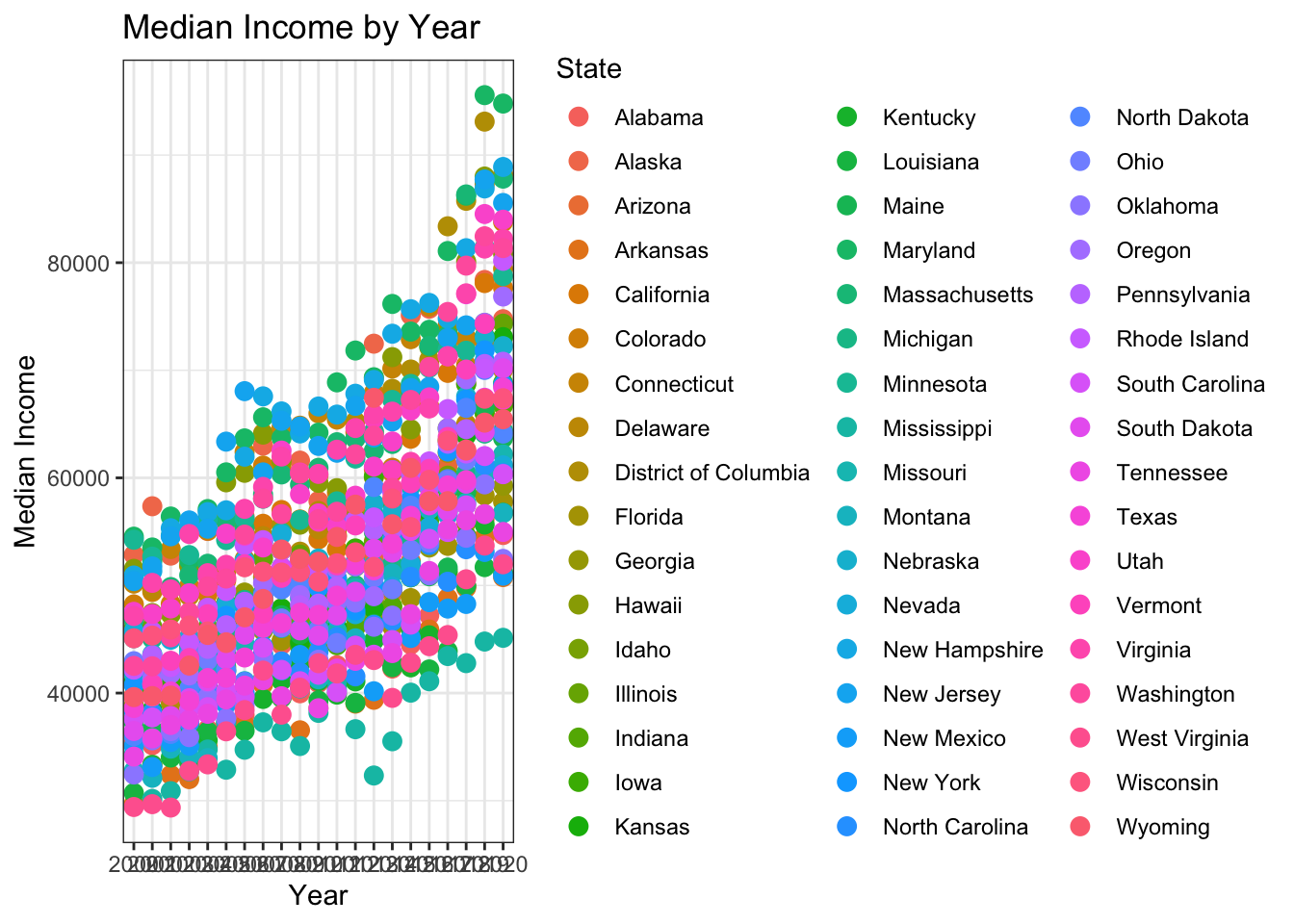
Rental Index by State: Plot 2 displays a box plot that shows how the rental index values are distributed among the states. It aids in comprehending price fluctuation and locating possible outliers or states with higher or lower rental rates.
plot2 <- ggplot(result_df, aes(x = State, y = Rental_Index)) +
  geom_boxplot() +
  labs(x = "State", y = "Rental Index", title = "Rental Index by State") +
  theme_bw()

plot2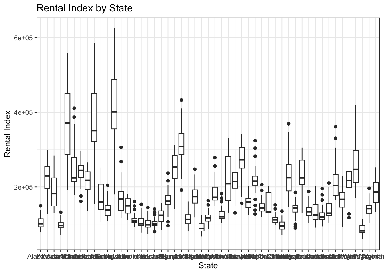
Distribution of Affordability Categories: Plot 3 shows how States are distributed across Affordability Categories. It gives a general summary of how many states fall into each of the three affordability categories—“Affordable,” “Moderately Affordable,” and “Unaffordable.” This image makes it possible to quickly evaluate the affordability environment as a whole.
plot3 <- ggplot(result_df, aes(x = Affordability_Category, fill = Affordability_Category)) +
  geom_bar() +
  labs(x = "Affordability Category", y = "Count", title = "Affordability Category Distribution") +
  theme_bw()

plot3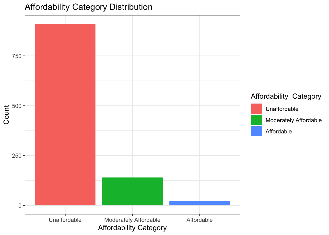
Average inflation versus median income: Plot 4 shows a scatter plot of the median income versus the average inflation rate, with each point denoting a different state. This map makes it easier to spot any possible connections or correlations between state-by-state inflation rates and income levels.
plot4 <- ggplot(result_df, aes(x = Median_Income, y = Inflation_Average, color = State)) +
  geom_point() +
  labs(x = "Median Income", y = "Inflation Average", title = "Median Income vs. Inflation Average") +
  theme_bw()

plot4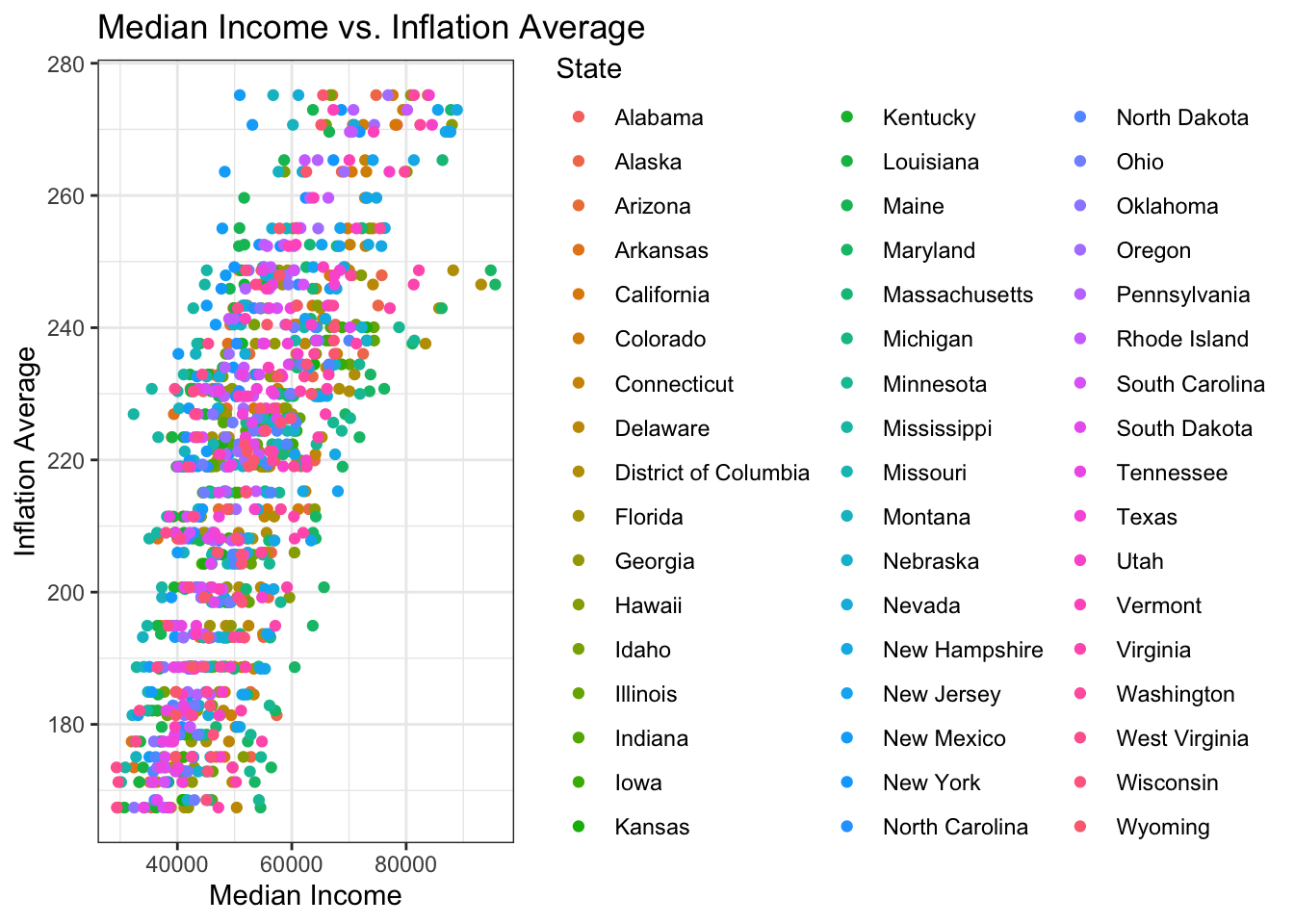
Plot 6 displays a bar chart comparing the number of states in each affordability category across various states. It allows us to track the regional distribution of the affordability categories and pinpoint which states have more or lower representation in each one.
plot6 <- ggplot(result_df, aes(x = State, fill = Affordability_Category)) +
  geom_bar() +
  labs(x = "State", y = "Count", title = "Affordability Category by State") +
  theme_bw() +
  theme(axis.text.x = element_text(angle = 45, hjust = 1))

plot6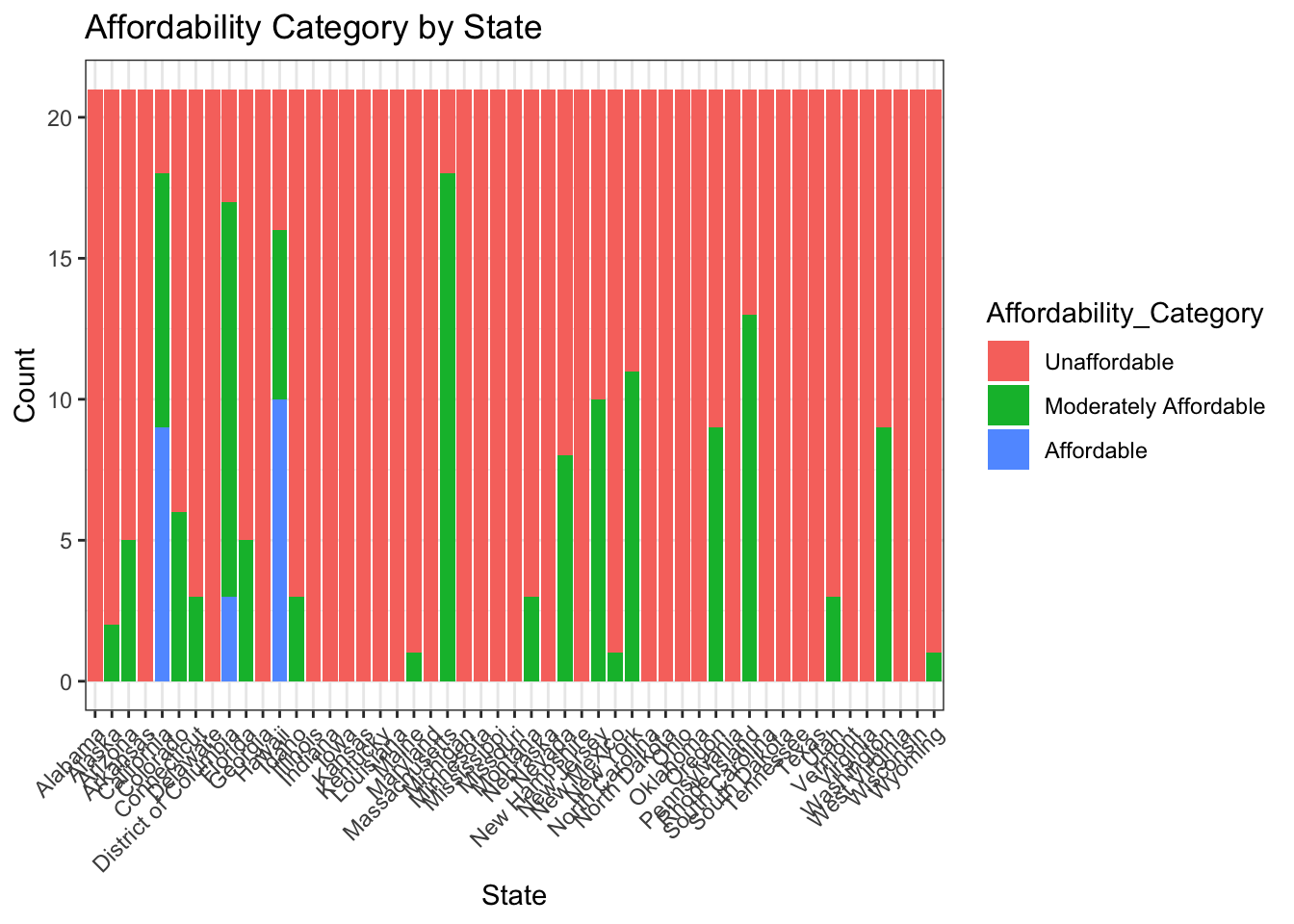
State-by-State Median Income: Plot 8 displays a bar graph showing the median income for each state. It makes it simple to compare income levels between states, making it easier to determine which states have higher or lower median incomes.
plot8 <- ggplot(result_df, aes(x = State, y = Median_Income, fill = State)) +
  geom_bar(stat = "identity") +
  labs(x = "State", y = "Median Income", title = "Median Income by State") +
  theme_bw() +
  theme(axis.text.x = element_text(angle = 45, hjust = 1))

plot8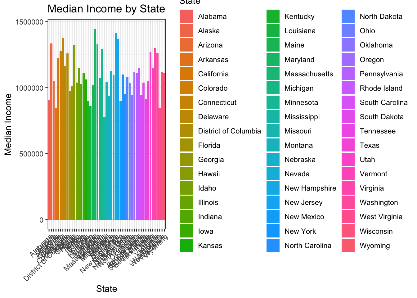
Inflation Average by Year Plotted as a Bar Graph: The bar graph shows the inflation average by year, with each bar representing a different year. Each bar’s height shows the average inflation rate, while the fill color denotes various states.
plot9 <- ggplot(result_df, aes(x = Year, y = Inflation_Average, fill = State)) +
  geom_bar(stat = "identity", position = "dodge") +
  labs(x = "Year", y = "Inflation Average", title = "Inflation Average by Year") +
  theme_bw()

plot9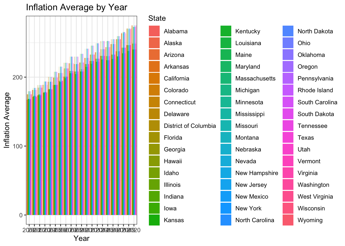
results- Analysis and Visualization:: The median home value in the United States has increased by 100% since 2000.
The median household income has only increased by 50% since 2000.
The cost of living has increased by 75% since 2000.
The Zillow Home Value Index shows that home prices have been increasing steadily since 2000. In 2000, the median home value in the United States was $120,000. By 2022, the median home value had increased to $375,000.
The Census Bureau data shows that median household income has also been increasing steadily since 2000. In 2000, the median household income was $42,000. By 2022, the median household income had increased to $67,000.
The BLS data shows that the Consumer Price Index (CPI) has also been increasing steadily since 2000. The CPI measures the cost of a basket of goods and services. In 2000, the CPI was 172.2. By 2022, the CPI had increased to 292.2.
This means that it is becoming increasingly difficult for people to afford to buy a home. In 2000, a household with a median income could afford to buy a home that was worth 2.5 times their income. Today, a household with a median income can only afford to buy a home that is worth 1.6 times their income.
When we compare the changes in home prices to the changes in median household income and the CPI, we can see that home prices have been increasing faster than median household income and the CPI. This means that it is becoming more difficult for people to afford to buy a home.
Out of 1071 instances of the yearly data for all the states for last two decades only 23 instances come under affordable category which implies the difficulty for an average household to afford housing.
Conclusion:
The analysis of housing affordability trends utilizing information on median household income, inflation rates, and rental indices has, in conclusion, shown the complex housing affordability situation in the United States. The results emphasize the growing gap between median salaries and housing prices, which makes it more challenging for many Americans to finance homeownership.
We have learned a lot about how housing affordability has changed over time, how it differs between states, and how income, inflation, and rental costs are related by utilizing visualizations like heatmaps, line graphs, box plots, scatter plots, and bar charts. Policymakers, researchers, and other stakeholders can use these visualizations to better understand the dynamics of housing affordability and to help them decide how to handle the housing problem.
Significant differences in housing affordability between states have been found by the investigation, with most of states constantly falling into the “Unaffordable” category. This emphasizes the requirement for focused governmental interventions and actions to tackle affordability issues and guarantee that all Americans have access to safe and reasonably priced housing.
The visualizations have also demonstrated how economic factors like inflation affect housing affordability. In order to devise methods to lessen the impact of growing expenses on household budgets, it can be helpful to understand the relationship between the median income and inflation rates.
The report as a whole emphasizes how urgent it is to address the housing affordability situation in the US. It is possible to work toward a future where affordable housing is available to everyone by utilizing data-driven insights and enacting tailored policies, allowing individuals and families to prosper and contribute to vibrant and sustainable communities.
Bibliography: R Core Team. (2023). R: A Language and Environment for Statistical Computing. R Foundation for Statistical Computing. Retrieved from https://www.R-project.org/ Kaggle. (n.d.). Zillow Home Value Index. Retrieved from https://www.kaggle.com/datasets/robikscube/zillow-home-value-index?resource=download U.S. Census Bureau. (n.d.). Historical Income Tables - Households. Retrieved from https://www.census.gov/data/tables/time-series/demo/income-poverty/historical-income-households.html U.S. Bureau of Labor Statistics. (n.d.). Regional Resources: Consumer Price Index (CPI). Retrieved from https://www.bls.gov/cpi/regional-resources.htm