Data.world is a platform for data collaboration, analysis, and sharing designed to help teams and organizations discover, use, and publish high-quality data in different contexts such as sports. Sports are a fundamental aspect of human culture and have been practiced for thousands of years. They provide a platform for physical activity, competition, and entertainment. Swimming is one of the many sports that have gained popularity around the world due to its many health benefits and its inclusion in major international events like the Olympics. Swimming features a variety of events, including freestyle, breaststroke, backstroke, and butterfly. The world records for each event are continually being broken by exceptional athletes who push the limits of human performance.
The swimming events at the Olympic Games are a highly anticipated competition featuring some of the world’s top athletes. Swimmers compete in a variety of disciplines, including freestyle, breaststroke, backstroke, butterfly, and medley, with races ranging from 50 meters to 1500 meters. Because analyzing a vast number of swimming history records it is of the scope of this paper, we will focusn on The top 200 time swimming styles and answer the following research questions:
1.Are there any patterns or trends in the progression of swimming
world records over time? For example, are records being broken more
frequently in certain events or during certain time periods?

2.Is there a relationship between a swimmer's age, gender, or
nationality and their likelihood of breaking a world record? For
example, do younger or older swimmers tend to break records more
often than their peers?

3.How do different strokes or distances compare in terms of the
frequency and magnitude of world record breaking? For example, are
world records more likely to be broken in shorter or longer races,
or in certain stroke categories?

4.Have advancements in technology or changes in swimming equipment
had an impact on the frequency or magnitude of world record
breaking? For example, have swimsuits or other equipment innovations
led to more world records being broken in recent years?
Part 2. Describe the data set(s)
Top 200 times in swimming styles includes details such as the event names, swim times, and swim dates for each swimmer’s performance, as well as information about the team they represent, their full name, gender, birth date, rank order, city, country code, and duration of their swim. In this datase each row representing a different swimmer and each column containing a specific piece of information about that swimmer’s performance. The data appears to be sourced from various international swimming competitions, including the Olympic Games, the FINA World Championships, and national championships in different countries. This dataset could be used to analyze trends in the Men’s 100 Freestyle event over time, such as changes in performance or the dominance of certain countries or swimmers. It could also be used to compare and contrast the performance of different swimmers or teams across various competitions.
Present the descriptive information of the dataset(s)
This data set has records from 716 different swimmers from around the world who participated in 474 events at different times in history .
dim(df_swim)
[1] 5200 14
length(unique(df_swim$`Event Name`))
[1] 474
length(unique(df_swim$`Team Name`))
[1] 58
length(unique(df_swim$`Athlete Full Name`))
[1] 716
table(df_swim$`Event description`)
      Men 100 Backstroke LCM Male     Men 100 Breaststroke LCM Male
                              200                               200
       Men 100 Butterfly LCM Male        Men 100 Freestyle LCM Male
                              200                               200
      Men 1500 Freestyle LCM Male       Men 200 Backstroke LCM Male
                              200                               200
    Men 200 Breaststroke LCM Male        Men 200 Butterfly LCM Male
                              200                               200
       Men 200 Freestyle LCM Male           Men 200 Medley LCM Male
                              200                               200
       Men 400 Freestyle LCM Male           Men 400 Medley LCM Male
                              200                               200
       Men 800 Freestyle LCM Male   Women 100 Backstroke LCM Female
                              200                               200
Women 100 Breaststroke LCM Female    Women 100 Butterfly LCM Female
                              200                               200
   Women 100 Freestyle LCM Female   Women 1500 Freestyle LCM Female
                              200                               200
  Women 200 Backstroke LCM Female Women 200 Breaststroke LCM Female
                              200                               200
   Women 200 Butterfly LCM Female    Women 200 Freestyle LCM Female
                              200                               200
      Women 200 Medley LCM Female    Women 400 Freestyle LCM Female
                              200                               200
      Women 400 Medley LCM Female    Women 800 Freestyle LCM Female
                              200                               200
head(df_swim)
Conduct summary statistics of the dataset adn for the variable Swim time.
     index       Event Name         Swim time          Swim date
 Min.   :   0   Length:5200        Length:5200        Length:5200
 1st Qu.:1300   Class :character   Class :character   Class :character
 Median :2600   Mode  :character   Mode  :character   Mode  :character
 Mean   :2600
 3rd Qu.:3899
 Max.   :5199

                     Event description   Team Code
 Men 100 Backstroke LCM Male  : 200    USA    :1360
 Men 100 Breaststroke LCM Male: 200    AUS    : 637
 Men 100 Butterfly LCM Male   : 200    JPN    : 427
 Men 100 Freestyle LCM Male   : 200    CHN    : 377
 Men 1500 Freestyle LCM Male  : 200    GBR    : 314
 Men 200 Backstroke LCM Male  : 200    HUN    : 287
 (Other)                      :4000    (Other):1798
                      Team Name                Athlete Full Name Gender
 United States of America  :1360   LEDECKY, Katie       : 218    F:2600
 Australia                 : 637   HOSSZU, Katinka      : 129    M:2600
 Japan                     : 427   PHELPS, Michael      :  86
 People's Republic of China: 377   SJOESTROEM, Sarah    :  82
 Great Britain             : 314   SUN, Yang            :  78
 Hungary                   : 287   PALTRINIERI, Gregorio:  75
 (Other)                   :1798   (Other)              :4532
 Athlete birth date   Rank_Order               City       Country Code
 03-17-97: 218      1      :  26   Tokyo         : 611   USA    : 710
 05-03-89: 129      2      :  26   Budapest      : 585   JPN    : 671
 05-24-94: 105      3      :  26   Rome          : 420   HUN    : 599
 06-30-85:  86      4      :  26   Rio de Janeiro: 234   ITA    : 497
 08-17-93:  82      5      :  26   Gwangju       : 230   CHN    : 439
 12-01-91:  78      6      :  26   (Other)       :3118   AUS    : 391
 (Other) :4502      (Other):5044   NA's          :   2   (Other):1893
 Duration (hh:mm:ss:ff)
 Length:5200
 Class :character
 Mode  :character
fav_stats(df_swim$`Swim time`)
Error in fav_stats(df_swim$`Swim time`): could not find function "fav_stats"
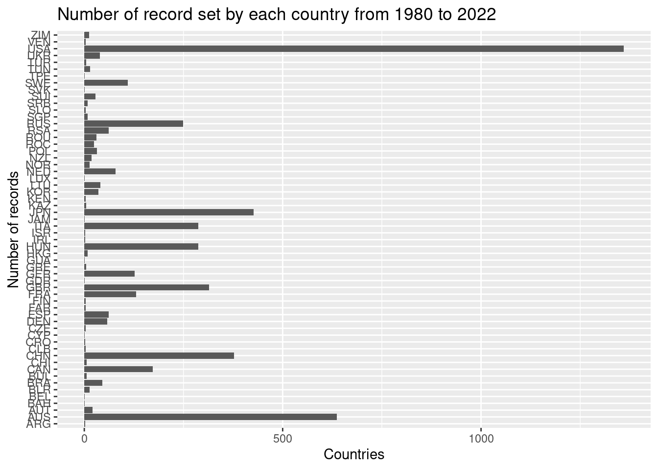
Let’s make quick view the number of record set by each country from 1980 to 2022.
p <-ggplot(df_swim, aes(x = df_swim$`Team Code`)) +geom_bar(stat ='count') +coord_flip() +labs(title ="Number of record set by each country from 1980 to 2022 ",x ="Number of records", y ="Countries")p
We can see that the dominant countries are The United States, Australia, Japan, China, and Great Britain. Our interest is not to analyse why they have the majority of records set from 1980 to 2022, but finding hidden patterns that can be evidenciated by data analysis.
To answer the first research question: Are there any patterns or trends in the progression of swimming world records over time? We can inspect the records being broken more frequently in certain events or during certain time periods.
The first step is to have a dedicated column with the year when the event took place. Let’s extract the year of the Swim Date column using the stringr library. This will facilitate and shorten the code implementation for the next research questions.
# extracting the event yeardate <-parse_date_time(df_swim$`Swim date`, orders ="mdy")# concatenating the years as a new columndf_swim$event_year =year(date)# sanity checkhead(df_swim)
sum(df_swim$event_year =="")
[1] 0
# extracting the athletes birth yeardate <-parse_date_time(df_swim$`Athlete birth date`, orders ="mdy")# concatenating the event_athle_age as a new columndf_swim$event_athle_age = df_swim$event_year -year(date)#sanity checkdf_swim
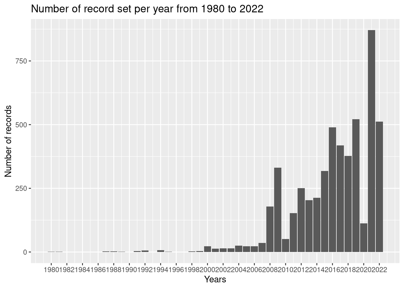
One interesting idea to investigate is whether the number of broken records is higher during certain time periods. To explore this, I plan to create a histogram of the years in which the most records were broken for specific events. This visualization will provide an overview of the trends in record-breaking across different time periods, which could potentially reveal patterns and help me draw meaningful conclusions from the data.
min_year <-min(df_swim$event_year)max_year <-max(df_swim$event_year)p <-ggplot(df_swim, aes(x = df_swim$event_year)) +geom_bar(stat ='count') +scale_x_continuous(breaks =seq(min_year, max_year, by =2 )) +labs(title ="Number of record set per year from 1980 to 2022 ",x ="Years", y ="Number of records")p
The data shows that from 1980 to 2020, swimmers of different ages, nationalities, and categories have continuously set new world records, pushing the limits of the discipline. In order to gain a deeper understanding of this trend, I plan to analyze the years 2008, 2009, 2016, 2019, and 2021, and observe which swimming events have set the most new records, regardless of nationality, gender, or age. By doing so, I hope to uncover patterns that may reveal whether certain time periods are associated with more frequent record-breaking. In addition, I plan to create a histogram of the years in which the most records were broken for specific events, which will provide a useful visual representation of the trends in record-breaking across different time periods.
min_age <-14max_age <-20# Filter the data to include only participants aged 14 to 20filtered_data <- df_swim %>%filter( df_swim$event_year ==2008| df_swim$event_year ==2009| df_swim$event_year ==2016| df_swim$event_year ==2019| df_swim$event_year ==2021 )print(filtered_data)
# A tibble: 2,390 × 16
   index `Event Name`    `Swim time` `Swim date` `Event description` `Team Code`
   <dbl> <chr>           <chr>       <chr>       <fct>               <fct>
 1     1 13th FINA Worl… 46.91       07-30-09    Men 100 Freestyle … BRA
 2     2 French Nationa… 46.94       04-23-09    Men 100 Freestyle … FRA
 3     3 18th FINA Worl… 46.96       07-25-19    Men 100 Freestyle … USA
 4     5 Olympic Games … 47.02       07-29-21    Men 100 Freestyle … USA
 5     6 Australian Nat… 47.04       04-10-16    Men 100 Freestyle … AUS
 6     7 Olympic Games … 47.05       08-13-08    Men 100 Freestyle … AUS
 7     9 Olympic Games … 47.08       07-29-21    Men 100 Freestyle … AUS
 8    10 18th FINA Worl… 47.08       07-25-19    Men 100 Freestyle … AUS
 9    11 13th FINA Worl… 47.09       07-26-09    Men 100 Freestyle … BRA
10    13 Olympic Games … 47.11       07-28-21    Men 100 Freestyle … ROC
# ℹ 2,380 more rows
# ℹ 10 more variables: `Team Name` <fct>, `Athlete Full Name` <fct>,
#   Gender <fct>, `Athlete birth date` <fct>, Rank_Order <fct>, City <fct>,
#   `Country Code` <fct>, `Duration (hh:mm:ss:ff)` <chr>, event_year <dbl>,
#   event_athle_age <dbl>
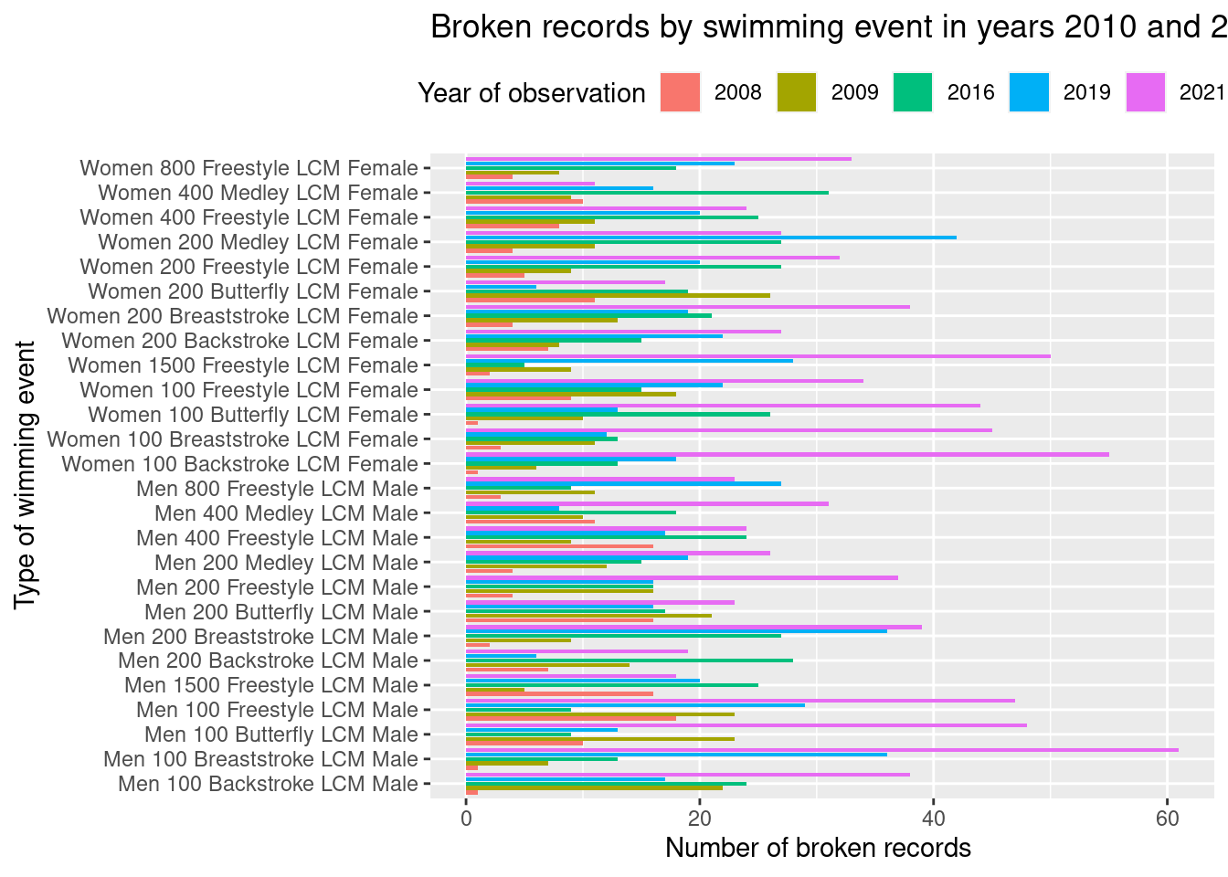
filtered_data <- filtered_data %>%mutate(event_year =factor(event_year))p <-ggplot(filtered_data, aes(`Event description`, fill = event_year)) +geom_histogram(stat ="count",position="dodge2") +theme(legend.position ="top") +coord_flip() +labs(x ="Type of wimming event", y ="Number of broken records ", title ="Broken records by swimming event in years 2010 and 2021") +guides(fill =guide_legend(title ="Year of observation"))p
By analyzing the years 2008, 2009, 2016, 2019, and 2021, I have observed that short swimming events, have been broken more frequently during this periods. Furthermore, specific swimming events such as the Women’s 100-meter Backstroke and the Men’s 100-meter Breaststroke are particularly representative of this pattern. By identifying such trends, I hope to gain a deeper understanding of the factors that contribute to record-breaking in swimming and how it has evolved over time.
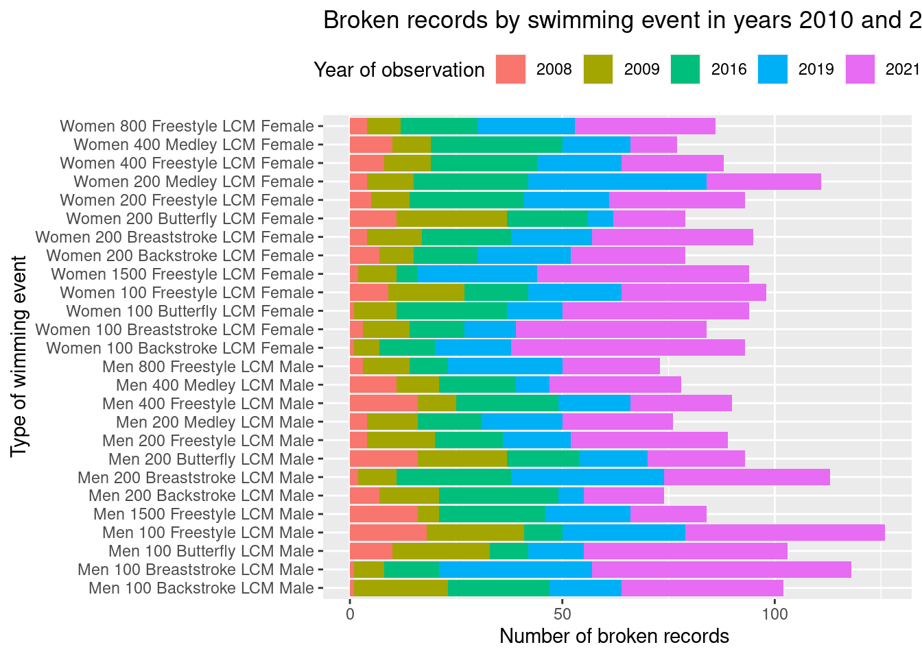
Another view of this pattern we found.
# Create a histogram of the filtered datap <-ggplot(filtered_data, aes(x =filtered_data$`Event description` )) +#geom_bar(stat = "count") +geom_bar(aes(fill= filtered_data$event_year), position =position_stack(reverse =TRUE)) +theme(legend.position ="top") +coord_flip() +labs(x ="Type of wimming event", y ="Number of broken records ", title ="Broken records by swimming event in years 2010 and 2021") +guides(fill =guide_legend(title ="Year of observation"))p
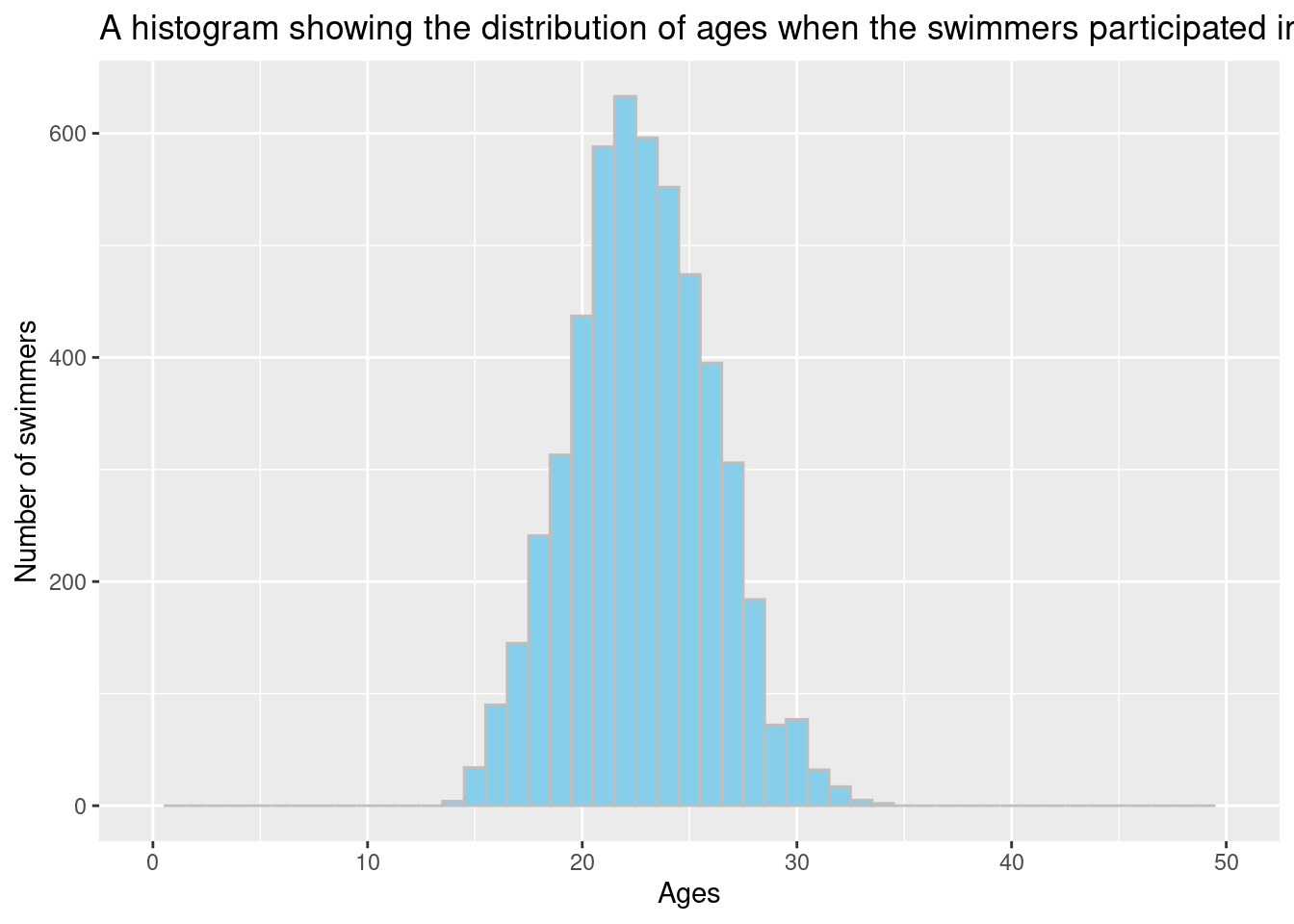
To investigates the relationship between a swimmer’s age, gender, or nationality and their likelihood of breaking a world record, requires several conditions to be met. These conditions include filtering the data by the same age, event name, team, and gender. After preprocessing the data, the distribution of ages of each swimmer at the year of the competition will be checked, and the ages of top records that participated in different events over time will be visualized. By following this plan, we can analyze the data and determine what are the possible trends.
Let’s plot a histogram
p <-ggplot(df_swim, aes(x = df_swim$event_athle_age)) +geom_histogram(binwidth =1, fill ="skyblue", color ="gray",show.legend =TRUE) +xlim(0,50) +labs(title ="A histogram showing the distribution of ages when the swimmers participated in a contest",x ="Ages", y ="Number of swimmers")p
The distribution of ages follows a bell-shaped curve which suggests that it is normally distributed. Observing the histogram, younger and older swimmers tend to break records.
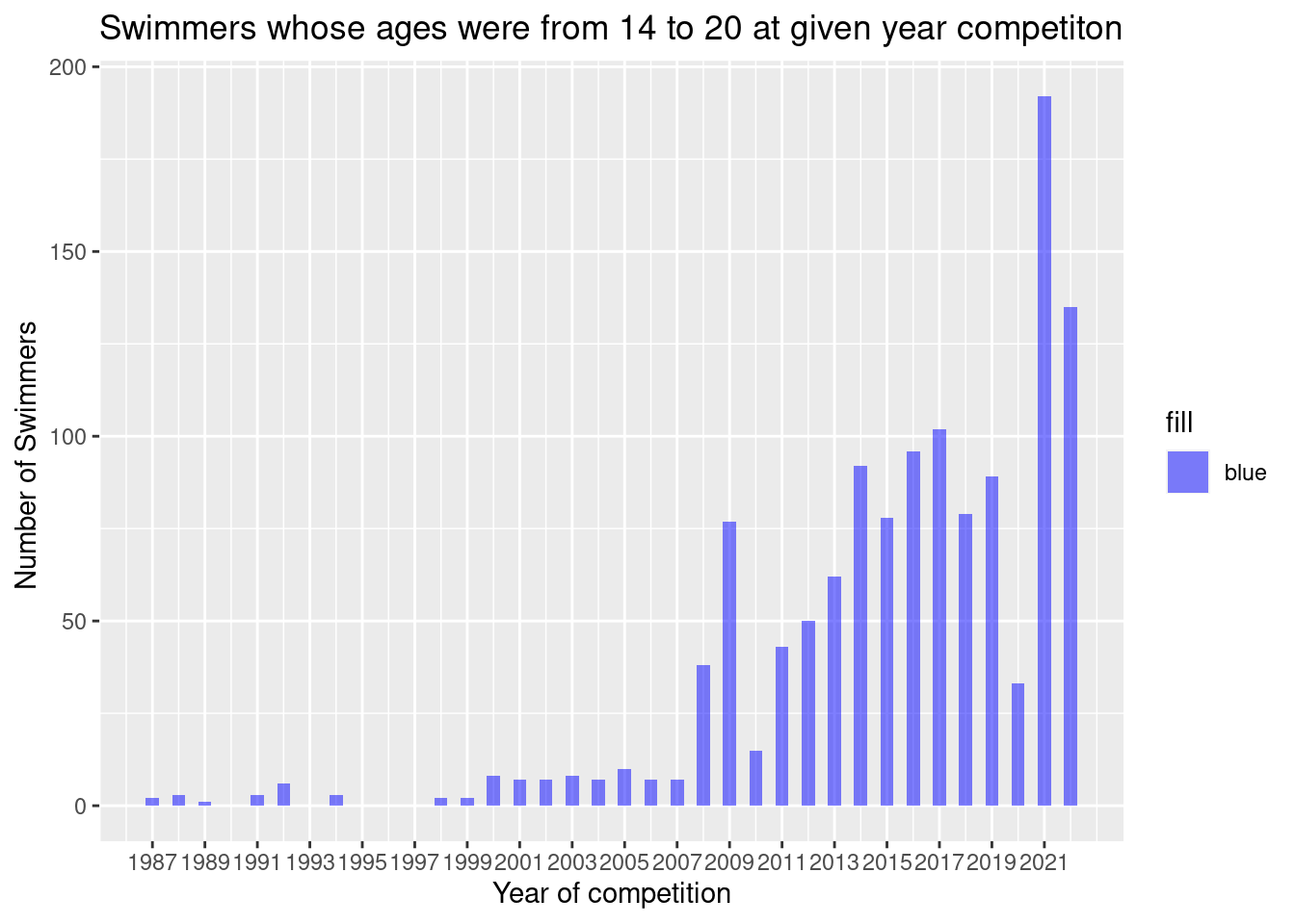
min_age <-14max_age <-20# Filter the data to include only participants aged 14 to 20filtered_data <- df_swim %>%filter( (df_swim$event_athle_age) >= min_age & (df_swim$event_athle_age) <= max_age)print(filtered_data)
# A tibble: 1,264 × 16
   index `Event Name`    `Swim time` `Swim date` `Event description` `Team Code`
   <dbl> <chr>           <chr>       <chr>       <fct>               <fct>
 1     0 European Champ… 46.86       08-13-22    Men 100 Freestyle … ROU
 2     4 European Champ… 46.98       08-12-22    Men 100 Freestyle … ROU
 3     8 8th FINA World… 47.07       08-30-22    Men 100 Freestyle … ROU
 4    15 19th FINA Worl… 47.13       06-21-22    Men 100 Freestyle … ROU
 5    17 European Champ… 47.20       08-12-22    Men 100 Freestyle … ROU
 6    27 European Junio… 47.30       07-08-21    Men 100 Freestyle … ROU
 7    35 8th FINA World… 47.37       08-30-22    Men 100 Freestyle … ROU
 8    49 14th FINA Worl… 47.49       07-24-11    Men 100 Freestyle … AUS
 9    62 European Junio… 47.54       07-05-22    Men 100 Freestyle … ROU
10    64 19th FINA Worl… 47.55       06-21-22    Men 100 Freestyle … CAN
# ℹ 1,254 more rows
# ℹ 10 more variables: `Team Name` <fct>, `Athlete Full Name` <fct>,
#   Gender <fct>, `Athlete birth date` <fct>, Rank_Order <fct>, City <fct>,
#   `Country Code` <fct>, `Duration (hh:mm:ss:ff)` <chr>, event_year <dbl>,
#   event_athle_age <dbl>
min_year <-min(filtered_data$event_year)max_year <-max(filtered_data$event_year)# Create a histogram of the filtered dataggplot(filtered_data, aes(x = filtered_data$event_year, fill ="blue")) +geom_histogram(binwidth = .5, alpha =0.5, position ="identity") +scale_x_continuous(breaks =seq(min_year, max_year, by =2 )) +scale_fill_manual(values ="blue") +labs(x ="Year of competition", y ="Number of Swimmers ", title ="Swimmers whose ages were from 14 to 20 at given year competiton")
Let’s show how the performance of the top 200 swimming styles in 100-meters free style have progressed in time per country.
3. The Tentative Plan for Visualization
Briefly describe what data analyses (please the special note on statistics in the next section) and visualizations you plan to conduct to answer the research questions you proposed above.
Explain why you choose to conduct these specific data analyses and visualizations. In other words, how do such types of statistics or graphs (see the R Gallery) help you answer specific questions? For example, how can a bivariate visualization reveal the relationship between two variables, or how does a linear graph of variables over time present the pattern of development?
If you plan to conduct specific data analyses and visualizations, describe how do you need to process and prepare the tidy data.
What do you need to do to mutate the datasets (convert date data, create a new variable, pivot the data format, etc.)?
How are you going to deal with the missing data/NAs and outliers? And why do you choose this way to deal with NAs?
(Optional) It is encouraged, but optional, to include a coding component of tidy data in this part.
References
- For reference, you can check out [the source of the dataset](https://data.world/romanian-data/swimming-dataset-top-200-world-times)
Source Code
---title: "Final Project Assignment#1: Kevin Martell Luya"author: "Kevin Martell Luya"description: "Project & Data Description"date: "04/25/2023"format: html: df-print: paged toc: true code-copy: true code-tools: true css: styles.csscategories: - final_Project_assignment_1 - final_project_data_descriptioneditor_options: chunk_output_type: consoleeditor: markdown: wrap: 72---```{r}#| label: setup#| warning: false#| message: falselibrary(tidyverse)library(ggplot2)library(here)library(mosaic)library(lubridate)library(stringr)knitr::opts_chunk$set(echo =TRUE, warning=FALSE, message=FALSE)```## Part 1. Introduction {#describe-the-data-sets}Data.world is a platform for data collaboration, analysis, and sharingdesigned to help teams and organizations discover, use, and publishhigh-quality data in different contexts such as sports. Sports are a fundamental aspect of human culture and have been practiced for thousands of years. They provide a platform for physical activity, competition, and entertainment. Swimming is one of the many sports that have gained popularity around the world due to its many health benefits and its inclusion in major international events like the Olympics. Swimming features a variety of events, including freestyle, breaststroke, backstroke, and butterfly. The world records for each event are continually being broken by exceptional athletes who push the limits of human performance.The swimming events at the Olympic Games are a highly anticipatedcompetition featuring some of the world's top athletes. Swimmers competein a variety of disciplines, including freestyle, breaststroke,backstroke, butterfly, and medley, with races ranging from 50 meters to1500 meters. Because analyzing a vast number of swimming history records it is of the scope of this paper, we will focusn on The top 200 time swimming styles and answer the following research questions: 1.Are there any patterns or trends in the progression of swimming world records over time? For example, are records being broken more frequently in certain events or during certain time periods? 2.Is there a relationship between a swimmer's age, gender, or nationality and their likelihood of breaking a world record? For example, do younger or older swimmers tend to break records more often than their peers? 3.How do different strokes or distances compare in terms of the frequency and magnitude of world record breaking? For example, are world records more likely to be broken in shorter or longer races, or in certain stroke categories? 4.Have advancements in technology or changes in swimming equipment had an impact on the frequency or magnitude of world record breaking? For example, have swimsuits or other equipment innovations led to more world records being broken in recent years?## Part 2. Describe the data set(s) {#describe-the-data-sets-1}Top 200 times in swimming styles includes details such as the event names, swim times, and swim dates for each swimmer's performance, as well as information about the team they represent, their full name, gender, birth date, rank order, city, country code, and duration of their swim. In this datase each row representing a different swimmer and each column containing a specific piece of information about that swimmer's performance. The data appears to be sourced from various international swimming competitions, including the Olympic Games, the FINA World Championships, and national championships in different countries.This dataset could be used to analyze trends in the Men's 100 Freestyle event over time, such as changes in performance or the dominance of certain countries or swimmers. It could also be used to compare and contrast the performance of different swimmers or teams across various competitions.1. Read the dataset```{r}df_swim<-read_csv("./_data/swimming_database.csv")df_swim```2. Present the descriptive information of the dataset(s) This data set has records from 716 different swimmers from around the world who participated in 474 events at different times in history .```{r}dim(df_swim)length(unique(df_swim$`Event Name`))length(unique(df_swim$`Team Name`))length(unique(df_swim$`Athlete Full Name`))table(df_swim$`Event description`)head(df_swim)```3. Conduct summary statistics of the dataset adn for the variable Swim time.```{r}df_swim <- df_swim %>%mutate(#`Event Name` = factor(`Event Name`),#`Swim time` = factor(`Swim time`),#`Swim date` = factor(`Swim date`),`Event description`=factor(`Event description`),`Team Code`=factor(`Team Code`),`Team Name`=factor(`Team Name`),`Athlete Full Name`=factor(`Athlete Full Name`),`Gender`=factor(`Gender`),`Athlete birth date`=factor(`Athlete birth date`),`Rank_Order`=factor(`Rank_Order`),`City`=factor(`City`),`Country Code`=factor(`Country Code`),#`Duration (hh:mm:ss:ff)` = factor(`Duration (hh:mm:ss:ff)`) )summary(df_swim)fav_stats(df_swim$`Swim time`)```Let's make quick view the number of record set by each country from 1980 to 2022.```{r}p <-ggplot(df_swim, aes(x = df_swim$`Team Code`)) +geom_bar(stat ='count') +coord_flip() +labs(title ="Number of record set by each country from 1980 to 2022 ",x ="Number of records", y ="Countries")p```We can see that the dominant countries are The United States, Australia, Japan, China, and Great Britain. Our interest is not to analyse why they have the majority of records set from 1980 to 2022, but finding hidden patterns that can be evidenciated by data analysis.To answer the first research question: Are there any patterns or trends in the progression of swimming world records over time? We can inspect the records being broken more frequently in certain events or during certain time periods. The first step is to have a dedicated column with the year when the event took place. Let's extract the year of the Swim Date column using the stringr library. This will facilitate and shorten the code implementation for the next research questions.```{r}# extracting the event yeardate <-parse_date_time(df_swim$`Swim date`, orders ="mdy")# concatenating the years as a new columndf_swim$event_year =year(date)# sanity checkhead(df_swim)sum(df_swim$event_year =="")# extracting the athletes birth yeardate <-parse_date_time(df_swim$`Athlete birth date`, orders ="mdy")# concatenating the event_athle_age as a new columndf_swim$event_athle_age = df_swim$event_year -year(date)#sanity checkdf_swim```One interesting idea to investigate is whether the number of broken records is higher during certain time periods. To explore this, I plan to create a histogram of the years in which the most records were broken for specific events. This visualization will provide an overview of the trends in record-breaking across different time periods, which could potentially reveal patterns and help me draw meaningful conclusions from the data.```{r}min_year <-min(df_swim$event_year)max_year <-max(df_swim$event_year)p <-ggplot(df_swim, aes(x = df_swim$event_year)) +geom_bar(stat ='count') +scale_x_continuous(breaks =seq(min_year, max_year, by =2 )) +labs(title ="Number of record set per year from 1980 to 2022 ",x ="Years", y ="Number of records")p```The data shows that from 1980 to 2020, swimmers of different ages, nationalities, and categories have continuously set new world records, pushing the limits of the discipline. In order to gain a deeper understanding of this trend, I plan to analyze the years 2008, 2009, 2016, 2019, and 2021, and observe which swimming events have set the most new records, regardless of nationality, gender, or age. By doing so, I hope to uncover patterns that may reveal whether certain time periods are associated with more frequent record-breaking. In addition, I plan to create a histogram of the years in which the most records were broken for specific events, which will provide a useful visual representation of the trends in record-breaking across different time periods.```{r}min_age <-14max_age <-20# Filter the data to include only participants aged 14 to 20filtered_data <- df_swim %>%filter( df_swim$event_year ==2008| df_swim$event_year ==2009| df_swim$event_year ==2016| df_swim$event_year ==2019| df_swim$event_year ==2021 )print(filtered_data)filtered_data <- filtered_data %>%mutate(event_year =factor(event_year))p <-ggplot(filtered_data, aes(`Event description`, fill = event_year)) +geom_histogram(stat ="count",position="dodge2") +theme(legend.position ="top") +coord_flip() +labs(x ="Type of wimming event", y ="Number of broken records ", title ="Broken records by swimming event in years 2010 and 2021") +guides(fill =guide_legend(title ="Year of observation"))p ```By analyzing the years 2008, 2009, 2016, 2019, and 2021, I have observed that short swimming events, have been broken more frequently during this periods. Furthermore, specific swimming events such as the Women's 100-meter Backstroke and the Men's 100-meter Breaststroke are particularly representative of this pattern. By identifying such trends, I hope to gain a deeper understanding of the factors that contribute to record-breaking in swimming and how it has evolved over time.Another view of this pattern we found. ```{r}# Create a histogram of the filtered datap <-ggplot(filtered_data, aes(x =filtered_data$`Event description` )) +#geom_bar(stat = "count") +geom_bar(aes(fill= filtered_data$event_year), position =position_stack(reverse =TRUE)) +theme(legend.position ="top") +coord_flip() +labs(x ="Type of wimming event", y ="Number of broken records ", title ="Broken records by swimming event in years 2010 and 2021") +guides(fill =guide_legend(title ="Year of observation"))p```To investigates the relationship between a swimmer's age, gender, or nationality and their likelihood of breaking a world record, requires several conditions to be met. These conditions include filtering the data by the same age, event name, team, and gender. After preprocessing the data, the distribution of ages of each swimmer at the year of the competition will be checked, and the ages of top records that participated in different events over time will be visualized. By following this plan, we can analyze the data and determine what are the possible trends.Let's plot a histogram```{r}p <-ggplot(df_swim, aes(x = df_swim$event_athle_age)) +geom_histogram(binwidth =1, fill ="skyblue", color ="gray",show.legend =TRUE) +xlim(0,50) +labs(title ="A histogram showing the distribution of ages when the swimmers participated in a contest",x ="Ages", y ="Number of swimmers")p```The distribution of ages follows a bell-shaped curve which suggests that it is normally distributed. Observing the histogram, younger and older swimmers tend to break records.```{r}min_age <-14max_age <-20# Filter the data to include only participants aged 14 to 20filtered_data <- df_swim %>%filter( (df_swim$event_athle_age) >= min_age & (df_swim$event_athle_age) <= max_age)print(filtered_data)min_year <-min(filtered_data$event_year)max_year <-max(filtered_data$event_year)# Create a histogram of the filtered dataggplot(filtered_data, aes(x = filtered_data$event_year, fill ="blue")) +geom_histogram(binwidth = .5, alpha =0.5, position ="identity") +scale_x_continuous(breaks =seq(min_year, max_year, by =2 )) +scale_fill_manual(values ="blue") +labs(x ="Year of competition", y ="Number of Swimmers ", title ="Swimmers whose ages were from 14 to 20 at given year competiton")```Let's show how the performance of the top 200 swimming styles in 100-meters free stylehave progressed in time per country.```{r}```## 3. The Tentative Plan for Visualization {#the-tentative-plan-for-visualization}1. Briefly describe what data analyses (**please the special note on statistics in the next section)** and visualizations you plan to conduct to answer the research questions you proposed above.2. Explain why you choose to conduct these specific data analyses and visualizations. In other words, how do such types of statistics or graphs (see [the R Gallery](https://r-graph-gallery.com/)) help you answer specific questions? For example, how can a bivariate visualization reveal the relationship between two variables, or how does a linear graph of variables over time present the pattern of development?3. If you plan to conduct specific data analyses and visualizations, describe how do you need to process and prepare the tidy data. - What do you need to do to mutate the datasets (convert date data, create a new variable, pivot the data format, etc.)? - How are you going to deal with the missing data/NAs and outliers? And why do you choose this way to deal with NAs?4. (Optional) It is encouraged, **but optional**, to include a coding component of tidy data in this part.## References - For reference, you can check out [the source of the dataset](https://data.world/romanian-data/swimming-dataset-top-200-world-times)