Challenge 4: FedFundRate.csv Clean Up

challenge_4

fed_rates

laurenzichittella

More data wrangling: pivoting

Author

Lauren Zichittella

Published

March 22, 2023

Code

library(tidyverse)

knitr::opts_chunk$set(echo = TRUE, warning=FALSE, message=FALSE)

Read in data

Read in FedFundRate.csv and utilize functions to understand dataset and formulate next steps in clean-up

Steps

Import data set. Utilize functions to understand data structure
Recreate data with better named columns to faciliate easier processing downstream
Utilize “sanity checks” to confirm no errors in logic or understanding
Output basic characterization of dataset

Next stepts

Create tidy version of dataset where each row represents a distinct date and type measurement
Further characterize data to inform any additional cleaning to be done and start planning for graphical display

Code

# Read in dataset and evaluate basics to understand any necessary basic cleanings that should be done before tidying

   fedfundrate_raw <-read_csv("_data/FedFundsRate.csv")
   colnames(fedfundrate_raw)

 [1] "Year"                         "Month"                       
 [3] "Day"                          "Federal Funds Target Rate"   
 [5] "Federal Funds Upper Target"   "Federal Funds Lower Target"  
 [7] "Effective Federal Funds Rate" "Real GDP (Percent Change)"   
 [9] "Unemployment Rate"            "Inflation Rate"

Code

   head(fedfundrate_raw)

# A tibble: 6 × 10
   Year Month   Day Federal Fu…¹ Feder…² Feder…³ Effec…⁴ Real …⁵ Unemp…⁶ Infla…⁷
  <dbl> <dbl> <dbl>        <dbl>   <dbl>   <dbl>   <dbl>   <dbl>   <dbl>   <dbl>
1  1954     7     1           NA      NA      NA    0.8      4.6     5.8      NA
2  1954     8     1           NA      NA      NA    1.22    NA       6        NA
3  1954     9     1           NA      NA      NA    1.06    NA       6.1      NA
4  1954    10     1           NA      NA      NA    0.85     8       5.7      NA
5  1954    11     1           NA      NA      NA    0.83    NA       5.3      NA
6  1954    12     1           NA      NA      NA    1.28    NA       5        NA
# … with abbreviated variable names ¹`Federal Funds Target Rate`,
#   ²`Federal Funds Upper Target`, ³`Federal Funds Lower Target`,
#   ⁴`Effective Federal Funds Rate`, ⁵`Real GDP (Percent Change)`,
#   ⁶`Unemployment Rate`, ⁷`Inflation Rate`

Code

   tail(fedfundrate_raw)

# A tibble: 6 × 10
   Year Month   Day Federal Fu…¹ Feder…² Feder…³ Effec…⁴ Real …⁵ Unemp…⁶ Infla…⁷
  <dbl> <dbl> <dbl>        <dbl>   <dbl>   <dbl>   <dbl>   <dbl>   <dbl>   <dbl>
1  2016    12     1           NA    0.5     0.25    0.54      NA     4.7     2.2
2  2016    12    14           NA    0.75    0.5    NA         NA    NA      NA  
3  2017     1     1           NA    0.75    0.5     0.65      NA     4.8     2.3
4  2017     2     1           NA    0.75    0.5     0.66      NA     4.7     2.2
5  2017     3     1           NA    0.75    0.5    NA         NA    NA      NA  
6  2017     3    16           NA    1       0.75   NA         NA    NA      NA  
# … with abbreviated variable names ¹`Federal Funds Target Rate`,
#   ²`Federal Funds Upper Target`, ³`Federal Funds Lower Target`,
#   ⁴`Effective Federal Funds Rate`, ⁵`Real GDP (Percent Change)`,
#   ⁶`Unemployment Rate`, ⁷`Inflation Rate`

Code

# Create pre-tidy version of data, changing variable names to make easier to reference in code 
   fedfundrate_pretidy <-read_csv("_data/FedFundsRate.csv"
                    , skip =1
                    , col_names = c("year", "month", "day", "fedfunds_targetrate", "fedfunds_targetupper",  "fedfunds_targetlower","fedfunds_effectiverate", "realgdp_percentchange",   "unemployment_rate",    "inflation_rate"))
   
   # confirm updated read did not affect row count or column counts
   nrow(fedfundrate_raw)

[1] 904

Code

   nrow(fedfundrate_pretidy)

[1] 904

Code

   ncol(fedfundrate_raw)

[1] 10

Code

   ncol(fedfundrate_pretidy)

[1] 10

Code

# Output basic summary to describe dataset 
   
   # quick summary 
   print(summarytools::dfSummary(fedfundrate_pretidy, 
                        plain.ascii  = FALSE, 
                        style        = "grid", 
                        graph.magnif = 0.70, ),
      method = 'render',
      table.classes = 'table-condensed')

Data Frame Summary

fedfundrate_pretidy

Dimensions: 904 x 10
Duplicates: 0

year [numeric]

Mean (sd) : 1986.7 (17.2)
min ≤ med ≤ max:
1954 ≤ 1987.5 ≤ 2017
IQR (CV) : 28 (0)

64 distinct values

904 (100.0%)

0 (0.0%)

month [numeric]

Mean (sd) : 6.6 (3.5)
min ≤ med ≤ max:
1 ≤ 7 ≤ 12
IQR (CV) : 6 (0.5)

12 distinct values

904 (100.0%)

0 (0.0%)

day [numeric]

Mean (sd) : 3.6 (6.8)
min ≤ med ≤ max:
1 ≤ 1 ≤ 31
IQR (CV) : 0 (1.9)

29 distinct values

904 (100.0%)

0 (0.0%)

fedfunds_targetrate [numeric]

Mean (sd) : 5.7 (2.6)
min ≤ med ≤ max:
1 ≤ 5.5 ≤ 11.5
IQR (CV) : 4 (0.5)

63 distinct values

462 (51.1%)

442 (48.9%)

fedfunds_targetupper [numeric]

Mean (sd) : 0.3 (0.1)
min ≤ med ≤ max:
0.2 ≤ 0.2 ≤ 1
IQR (CV) : 0 (0.5)

4 distinct values

103 (11.4%)

801 (88.6%)

fedfunds_targetlower [numeric]

Mean (sd) : 0.1 (0.1)
min ≤ med ≤ max:
0 ≤ 0 ≤ 0.8
IQR (CV) : 0 (2.4)

4 distinct values

103 (11.4%)

801 (88.6%)

fedfunds_effectiverate [numeric]

Mean (sd) : 4.9 (3.6)
min ≤ med ≤ max:
0.1 ≤ 4.7 ≤ 19.1
IQR (CV) : 4.2 (0.7)

466 distinct values

752 (83.2%)

152 (16.8%)

realgdp_percentchange [numeric]

Mean (sd) : 3.1 (3.6)
min ≤ med ≤ max:
-10 ≤ 3.1 ≤ 16.5
IQR (CV) : 3.5 (1.1)

113 distinct values

250 (27.7%)

654 (72.3%)

unemployment_rate [numeric]

Mean (sd) : 6 (1.6)
min ≤ med ≤ max:
3.4 ≤ 5.7 ≤ 10.8
IQR (CV) : 2.1 (0.3)

71 distinct values

752 (83.2%)

152 (16.8%)

inflation_rate [numeric]

Mean (sd) : 3.7 (2.6)
min ≤ med ≤ max:
0.6 ≤ 2.8 ≤ 13.6
IQR (CV) : 2.7 (0.7)

106 distinct values

710 (78.5%)

194 (21.5%)

Generated by summarytools 1.0.1 (R version 4.2.2)
2023-03-22

Code

  # Confirm date distinct by row 
  fedfundrate_pretidy%>%
      select(year,month,day)%>%
             n_distinct()

[1] 904

Code

  # evaluate the count of records per year/month & distribution of day 
  fedfundrate_pretidy  %>%
    group_by(year,month) %>%
       summarise(   n = n()
                  , min(day, na.rm=T)
                  , max_day = max(day, na.rm=T))%>%
          arrange(year, month)

# A tibble: 753 × 5
# Groups:   year [64]
    year month     n `min(day, na.rm = T)` max_day
   <dbl> <dbl> <int>                 <dbl>   <dbl>
 1  1954     7     1                     1       1
 2  1954     8     1                     1       1
 3  1954     9     1                     1       1
 4  1954    10     1                     1       1
 5  1954    11     1                     1       1
 6  1954    12     1                     1       1
 7  1955     1     1                     1       1
 8  1955     2     1                     1       1
 9  1955     3     1                     1       1
10  1955     4     1                     1       1
# … with 743 more rows

Code

  # evaluate the missingness of measures by year;
    fedfundrate_pretidy  %>%
    group_by(year) %>%
       summarise( n = n(),
                  na_count_fedfunds_targetrate    = sum(is.na(fedfunds_targetrate )),
                  na_count_fedfunds_targetupper   = sum(is.na(fedfunds_targetupper)),
                  na_count_fedfunds_targetlower   = sum(is.na(fedfunds_targetlower)), 
                  na_count_fedfunds_effectiverate = sum(is.na(fedfunds_effectiverate )), 
                  na_count_realgdp_percentchange  = sum(is.na(realgdp_percentchange)), 
                  na_count_unemployment_rate      = sum(is.na(unemployment_rate )), 
                  na_count_inflation_rate         = sum(is.na(inflation_rate)) )

# A tibble: 64 × 9
    year     n na_count_fedfun…¹ na_co…² na_co…³ na_co…⁴ na_co…⁵ na_co…⁶ na_co…⁷
   <dbl> <int>             <int>   <int>   <int>   <int>   <int>   <int>   <int>
 1  1954     6                 6       6       6       0       4       0       6
 2  1955    12                12      12      12       0       8       0      12
 3  1956    12                12      12      12       0       8       0      12
 4  1957    12                12      12      12       0       8       0      12
 5  1958    12                12      12      12       0       8       0       0
 6  1959    12                12      12      12       0       8       0       0
 7  1960    12                12      12      12       0       8       0       0
 8  1961    12                12      12      12       0       8       0       0
 9  1962    12                12      12      12       0       8       0       0
10  1963    12                12      12      12       0       8       0       0
# … with 54 more rows, and abbreviated variable names
#   ¹na_count_fedfunds_targetrate, ²na_count_fedfunds_targetupper,
#   ³na_count_fedfunds_targetlower, ⁴na_count_fedfunds_effectiverate,
#   ⁵na_count_realgdp_percentchange, ⁶na_count_unemployment_rate,
#   ⁷na_count_inflation_rate

Code

   #evaluate mean and median measures by year 
   fedfundrate_pretidy  %>%
      group_by(year) %>%
         summarise(avg_fedfunds_targetrate = mean(fedfunds_targetrate, na.rm=TRUE),
                   med_fedfunds_targetrate = median(fedfunds_targetrate, na.rm=TRUE),
                 
                   avg_fedfunds_targetupper = mean(fedfunds_targetupper, na.rm=TRUE),
                   med_fedfunds_targetupper = median(fedfunds_targetupper, na.rm=TRUE),
                 
                   avg_fedfunds_targetlower = mean(fedfunds_targetlower, na.rm=TRUE),
                   med_fedfunds_targetlower = median(fedfunds_targetlower, na.rm=TRUE),
                 
                   avg_fedfunds_effectiverate = mean(fedfunds_effectiverate, na.rm=TRUE),
                   med_fedfunds_effectiverate = median(fedfunds_effectiverate, na.rm=TRUE),
                 
                   avg_realgdp_percentchange= mean(realgdp_percentchange, na.rm=TRUE),
                   med_realgdp_percentchange = median(realgdp_percentchange, na.rm=TRUE),
                 
                   avg_unemployment_rate = mean(unemployment_rate, na.rm=TRUE),
                   med_unemployment_rate = median(unemployment_rate, na.rm=TRUE),
                 
                   avg_inflation_rate = mean(inflation_rate, na.rm=TRUE),
                   med_inflation_rate = median(inflation_rate, na.rm=TRUE) )

# A tibble: 64 × 15
    year avg_f…¹ med_f…² avg_f…³ med_f…⁴ avg_f…⁵ med_f…⁶ avg_f…⁷ med_f…⁸ avg_r…⁹
   <dbl>   <dbl>   <dbl>   <dbl>   <dbl>   <dbl>   <dbl>   <dbl>   <dbl>   <dbl>
 1  1954     NaN      NA     NaN      NA     NaN      NA    1.01   0.955   6.3  
 2  1955     NaN      NA     NaN      NA     NaN      NA    1.78   1.66    6.62 
 3  1956     NaN      NA     NaN      NA     NaN      NA    2.73   2.74    2.08 
 4  1957     NaN      NA     NaN      NA     NaN      NA    3.10   3       0.425
 5  1958     NaN      NA     NaN      NA     NaN      NA    1.57   1.6     2.97 
 6  1959     NaN      NA     NaN      NA     NaN      NA    3.30   3.43    4.65 
 7  1960     NaN      NA     NaN      NA     NaN      NA    3.22   3.28    0.975
 8  1961     NaN      NA     NaN      NA     NaN      NA    1.96   1.99    6.35 
 9  1962     NaN      NA     NaN      NA     NaN      NA    2.71   2.82    4.32 
10  1963     NaN      NA     NaN      NA     NaN      NA    3.18   3.01    5.18 
# … with 54 more rows, 5 more variables: med_realgdp_percentchange <dbl>,
#   avg_unemployment_rate <dbl>, med_unemployment_rate <dbl>,
#   avg_inflation_rate <dbl>, med_inflation_rate <dbl>, and abbreviated
#   variable names ¹avg_fedfunds_targetrate, ²med_fedfunds_targetrate,
#   ³avg_fedfunds_targetupper, ⁴med_fedfunds_targetupper,
#   ⁵avg_fedfunds_targetlower, ⁶med_fedfunds_targetlower,
#   ⁷avg_fedfunds_effectiverate, ⁸med_fedfunds_effectiverate, …

Tidy Data

The FedFundsRate dataset is a wide data set. To make it tidy, the data will need to be pivoted long and a new variable created to represent the type of measure per observation.

Steps

Pivot data longer to create one observation per distinct date (month, day, year) and type of measurement. Evaluate pivot results in the to confirm results as expected, proper number of rows and columns
Drop records with missing value for measure
Evaluate distribution of day by measure, year and month. Drop if single measure per each category to simplify going forward
Evaluate frequency of records by measure type, year, and month to identify measures populated for sample time period to graph for analysis

Next steps

Create single date variable by concatenating month, day, and year into single variable
Mutate measure_varname to facilitate easier filtering to create graphics
Test out ggplot options for displaying data

Code

# Pivot longer to convert each measure to a row in the dataset #
fedfundrate_tidy <- 
  fedfundrate_pretidy %>%
      pivot_longer( cols = c("fedfunds_targetrate", "fedfunds_targetupper", "fedfunds_targetlower","fedfunds_effectiverate", "realgdp_percentchange",   "unemployment_rate",    "inflation_rate"), 
                   names_to = "measure_varname",
                   values_to = "measure_value",
                   values_drop_na = FALSE    )

   # View first and last obs of pivoted data
   head(fedfundrate_tidy)

# A tibble: 6 × 5
   year month   day measure_varname        measure_value
  <dbl> <dbl> <dbl> <chr>                          <dbl>
1  1954     7     1 fedfunds_targetrate             NA  
2  1954     7     1 fedfunds_targetupper            NA  
3  1954     7     1 fedfunds_targetlower            NA  
4  1954     7     1 fedfunds_effectiverate           0.8
5  1954     7     1 realgdp_percentchange            4.6
6  1954     7     1 unemployment_rate                5.8

Code

   tail(fedfundrate_tidy)

# A tibble: 6 × 5
   year month   day measure_varname        measure_value
  <dbl> <dbl> <dbl> <chr>                          <dbl>
1  2017     3    16 fedfunds_targetupper            1   
2  2017     3    16 fedfunds_targetlower            0.75
3  2017     3    16 fedfunds_effectiverate         NA   
4  2017     3    16 realgdp_percentchange          NA   
5  2017     3    16 unemployment_rate              NA   
6  2017     3    16 inflation_rate                 NA

Code

   # Evaluate pivot results to confirm valid 
      # row counts
      nrow(fedfundrate_raw)

[1] 904

Code

      nrow(fedfundrate_pretidy)

[1] 904

Code

      nrow(fedfundrate_tidy)

[1] 6328

Code

      # column counts
      ncol(fedfundrate_raw)

[1] 10

Code

      ncol(fedfundrate_pretidy)

[1] 10

Code

      ncol(fedfundrate_tidy)

[1] 5

Code

      # calculation check
      nrow(fedfundrate_pretidy) * 7

[1] 6328

Code

# Remove observations where measure value missing;
  fedfundrate_tidy <- 
     fedfundrate_tidy %>%
        filter(!is.na(measure_value))    

   # Capture change in row number, evaluate observations to confirm look as expected;
   nrow(fedfundrate_tidy)

[1] 3132

Code

   head(fedfundrate_tidy)

# A tibble: 6 × 5
   year month   day measure_varname        measure_value
  <dbl> <dbl> <dbl> <chr>                          <dbl>
1  1954     7     1 fedfunds_effectiverate          0.8 
2  1954     7     1 realgdp_percentchange           4.6 
3  1954     7     1 unemployment_rate               5.8 
4  1954     8     1 fedfunds_effectiverate          1.22
5  1954     8     1 unemployment_rate               6   
6  1954     9     1 fedfunds_effectiverate          1.06

Code

# Create table with frequency of day value  by measure, month, and year
   ggplot(fedfundrate_tidy,aes(x = year, y =measure_value, fill = measure_varname)) +
          geom_bar(stat = "identity", position = "dodge")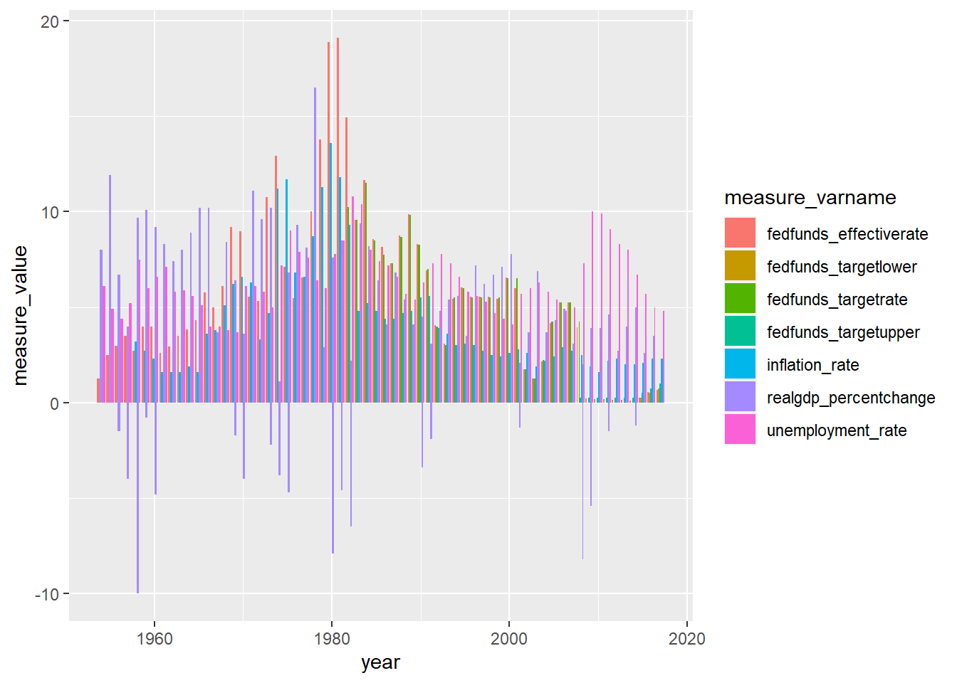

Mutate variables

Right now, type of measure is defined using one variable. I will mutate this single value to parse types in hopes of making graphics that are more focused. A single date variable will be created by concatenating what are now separatae columns for month, day, and year into single field. This will make displaying changes over time simpler to code. Finally, I will evaluate options for graphing results to inform best options for displaying relationship between measures or lack thereof.

Steps

Mutate measure_varname to create separate variable for measure type and measure calculation
Create single date variable from month, day, and year
Create histogram to evaluate values of percent change GDP and figure out how to display this measure alongside others
Utilize new variables to filter, plot data, figure out best choice to graph relationships across measures and types

Next steps:

Create final graphs to show relationship between federal fund rates & other measures

a - Federal funds line graph: rate, lower target, upper target b - Federal funds line graph: rate * (GDP, Inflation rate, Unemployment rate)

Conclusion

There is a lot of information in this dataset and it seems the best way to display is by plotting federal fund rate only, omiting target upper and lower because they are tightly correlated with the rate and their addition makes the visuals too dense.

Code

# Create two new variables to represent measure type and calculation 
   fedfundrate_tidy <- 
      fedfundrate_tidy %>% 
         separate(measure_varname, c("measure_type", "measure_calculation"), sep = "_") 

  # confirm variables created as intended. 
   head(fedfundrate_tidy)

# A tibble: 6 × 6
   year month   day measure_type measure_calculation measure_value
  <dbl> <dbl> <dbl> <chr>        <chr>                       <dbl>
1  1954     7     1 fedfunds     effectiverate                0.8 
2  1954     7     1 realgdp      percentchange                4.6 
3  1954     7     1 unemployment rate                         5.8 
4  1954     8     1 fedfunds     effectiverate                1.22
5  1954     8     1 unemployment rate                         6   
6  1954     9     1 fedfunds     effectiverate                1.06

Code

# Create single date field by combining variables month, day, and year 
   fedfundrate_tidy <- 
     fedfundrate_tidy %>% 
        mutate('measure_date' = make_date(year = year, month = month, day = day))
   
  # confirm variables created as intended.    
   head(fedfundrate_tidy)

# A tibble: 6 × 7
   year month   day measure_type measure_calculation measure_value measure_date
  <dbl> <dbl> <dbl> <chr>        <chr>                       <dbl> <date>      
1  1954     7     1 fedfunds     effectiverate                0.8  1954-07-01  
2  1954     7     1 realgdp      percentchange                4.6  1954-07-01  
3  1954     7     1 unemployment rate                         5.8  1954-07-01  
4  1954     8     1 fedfunds     effectiverate                1.22 1954-08-01  
5  1954     8     1 unemployment rate                         6    1954-08-01  
6  1954     9     1 fedfunds     effectiverate                1.06 1954-09-01

Code

# Remove columns for month, day, and year 
   fedfundrate_tidy <- 
     fedfundrate_tidy %>% 
          select(-year, -month, -day)
   
  # confirm variables removed as intended.   
   head(fedfundrate_tidy)

# A tibble: 6 × 4
  measure_type measure_calculation measure_value measure_date
  <chr>        <chr>                       <dbl> <date>      
1 fedfunds     effectiverate                0.8  1954-07-01  
2 realgdp      percentchange                4.6  1954-07-01  
3 unemployment rate                         5.8  1954-07-01  
4 fedfunds     effectiverate                1.22 1954-08-01  
5 unemployment rate                         6    1954-08-01  
6 fedfunds     effectiverate                1.06 1954-09-01

Code

# evaluate distribution of records and year across values of measure_type
   fedfundrate_tidy%>%
      group_by(measure_type)%>%
          summarise(num_records = n(),
                    min_measure_date    = min(measure_date),
                    max_measure_date    = max(measure_date))%>%
              arrange(desc(num_records))

# A tibble: 4 × 4
  measure_type num_records min_measure_date max_measure_date
  <chr>              <int> <date>           <date>          
1 fedfunds            1420 1954-07-01       2017-03-16      
2 unemployment         752 1954-07-01       2017-02-01      
3 inflation            710 1958-01-01       2017-02-01      
4 realgdp              250 1954-07-01       2016-10-01

Code

  # Look at histogram by measure calculation to evaluate distributions of rates versus percent change 
  ggplot(fedfundrate_tidy,
     aes(x = measure_value, color = measure_calculation)) +
     geom_density()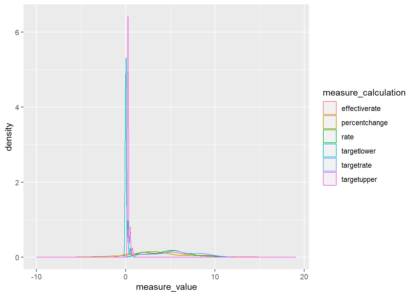

Code

# isolate federal fund fed funds effective rate plus non-fedfunds measure   
   fedfunds_graph <- 
      fedfundrate_tidy%>%
         filter(measure_type=="fedfunds" & measure_calculation == "effectiverate"| measure_type !="fedfunds"& measure_type !="realgdp")  
   
   head(fedfunds_graph)

# A tibble: 6 × 4
  measure_type measure_calculation measure_value measure_date
  <chr>        <chr>                       <dbl> <date>      
1 fedfunds     effectiverate                0.8  1954-07-01  
2 unemployment rate                         5.8  1954-07-01  
3 fedfunds     effectiverate                1.22 1954-08-01  
4 unemployment rate                         6    1954-08-01  
5 fedfunds     effectiverate                1.06 1954-09-01  
6 unemployment rate                         6.1  1954-09-01

Code

   # confirm correct records selected   
   fedfunds_graph%>%
      group_by (measure_type, measure_calculation )%>%
          summarise(num_records = n())

# A tibble: 3 × 3
# Groups:   measure_type [3]
  measure_type measure_calculation num_records
  <chr>        <chr>                     <int>
1 fedfunds     effectiverate               752
2 inflation    rate                        710
3 unemployment rate                        752

Code

# Create graph to show relationship between fed fund rate and other rate measures excluding % change GDP
   
   # bar chart - not great a great result. Next!
   ggplot(fedfunds_graph,aes(x = measure_date, y =measure_value, fill = measure_type)) +
          geom_bar(stat = "identity", position = "dodge")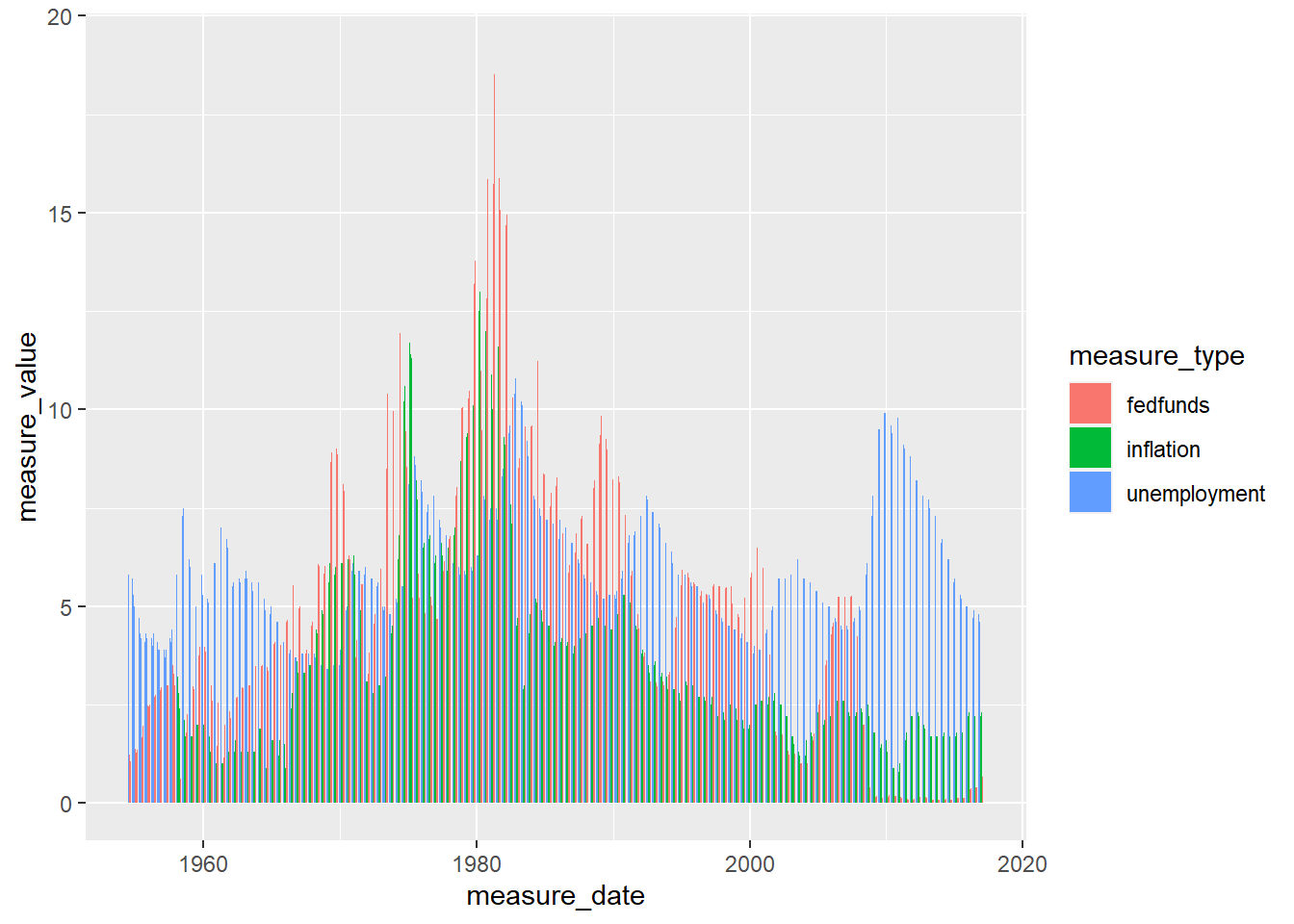

Code

   # line plot - this is better but hard to see trend. Next!
  ggplot(fedfunds_graph, aes(x=measure_date, y=measure_value, group=measure_type, color=measure_type)) +
    geom_line()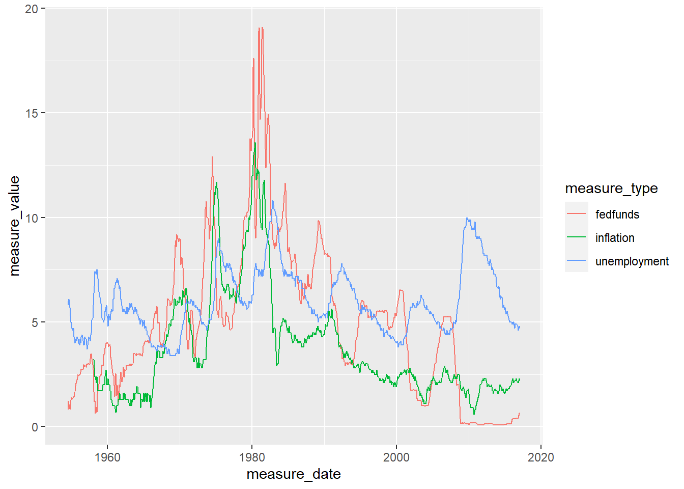

Code

  # line plot with regression line. That's much better! 
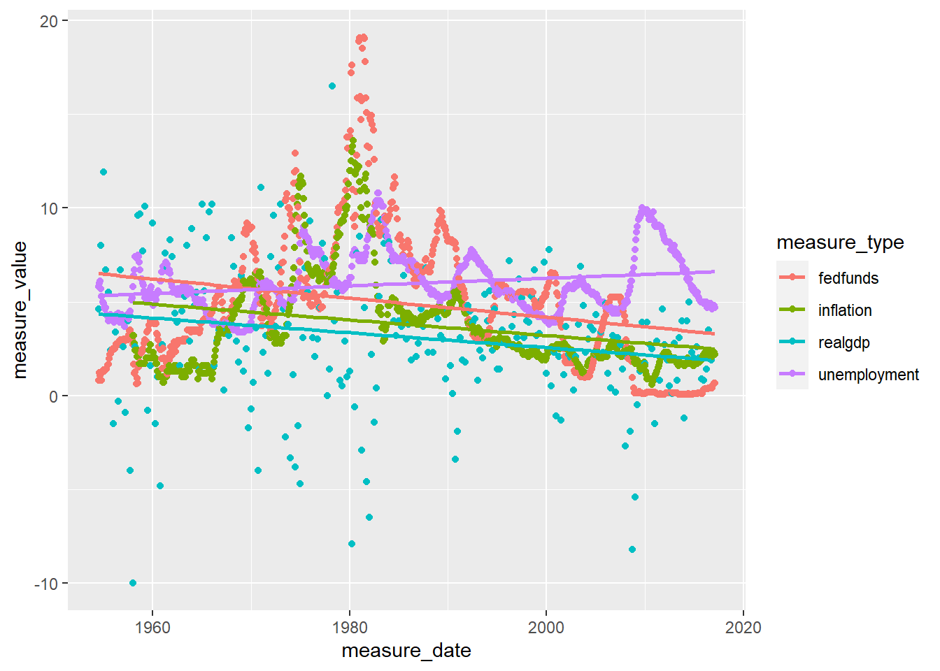
  ggplot(fedfunds_graph, aes(x = measure_date, y = measure_value, color = measure_type)) +
  geom_point() +
  geom_smooth(method = "lm", fill = NA)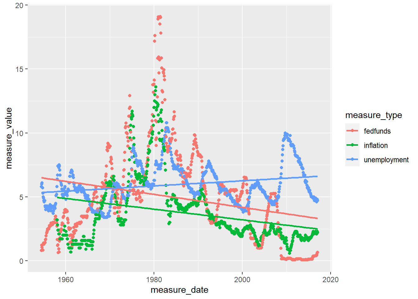

Data Description

The FedFundRates dataset provides measures of economic conditions in the US between July 1, 1954 and March 16, 2017. Each row of data represents a distinct date (month, day, year) and can include up to 6 measurements including: federal fund target rate, federal fund upper & lower target rates, federal fund lower target rate, federal funds effective rate, GDP percent change, unemployment rate, and inflation rate. However, variable are not populated consistently across observations

Graphs displayed below show the correlation between federal fund rates and measures for GDP, unemployment, and inflation. In short, how rates decrease alongside negative trends in economic health.

Code

# filter dataframe to retain federal fund effective, GDP, unemployment, and inflation rates
   fedfunds_final_graph <- 
      fedfundrate_tidy%>%
         filter(measure_type=="fedfunds" & measure_calculation == "effectiverate"| measure_type !="fedfunds") 
   
   # confirm correct records selected   
      fedfunds_final_graph%>%
         group_by (measure_type, measure_calculation )%>%
            summarise(num_records = n())

# A tibble: 4 × 3
# Groups:   measure_type [4]
  measure_type measure_calculation num_records
  <chr>        <chr>                     <int>
1 fedfunds     effectiverate               752
2 inflation    rate                        710
3 realgdp      percentchange               250
4 unemployment rate                        752

Code

      head(fedfunds_final_graph)

# A tibble: 6 × 4
  measure_type measure_calculation measure_value measure_date
  <chr>        <chr>                       <dbl> <date>      
1 fedfunds     effectiverate                0.8  1954-07-01  
2 realgdp      percentchange                4.6  1954-07-01  
3 unemployment rate                         5.8  1954-07-01  
4 fedfunds     effectiverate                1.22 1954-08-01  
5 unemployment rate                         6    1954-08-01  
6 fedfunds     effectiverate                1.06 1954-09-01

Code

  # line plot with regression line. That's much better! 
  ggplot(fedfunds_final_graph, aes(x = measure_date, y = measure_value, color = measure_type)) +
  geom_point() +
  geom_smooth(method = "lm", fill = NA)