Challenge 6: Visualizing USA Households Data

laurenzichittella

challenge_6

usa_households

Visualizing Time and Relationships

Author

Lauren Zichittella

Published

August 23, 2022

library(tidyverse)
library(ggplot2)

knitr::opts_chunk$set(echo = TRUE, warning=FALSE, message=FALSE)

Chunk 1: Read in data

The dataset I chose to utilize for this task measures the distribution of household income in the US between 1967 and 2019 by race and Hispanic origin.

During import of this file, I will limit observations to those that represent data by filtering out the header and footer sections. In addition, variables will be renamed from their original form in the xlsx file so new values are easier to understand and program with.

library(readxl)
library(stringr)

# Import data 
   usa_hh_raw <- read_excel( "_data/USA Households by Total Money Income, Race, and Hispanic Origin of Householder 1967 to 2019.xlsx"
                          , skip = 5
                          , col_names = c("hhorigin_year", "hh_n_k", "del", "pctdis_lt_15k", "pctdis_15_lt_25k", "pctdis_25_lt_35k", "pctdis_35_lt_50k", "pctdis_50_lt_75k", "pctdis_75_lt_100k","pctdis_100_lt_150k", "pctdis_150_lt_200k", "pctdis_ge_200k", "med_income", "me_med_income", "mean_income", "me_mean_income"))%>%
       select(!contains("del")) 

# remove footers obs  
   usa_hh_tidier <- 
         head(usa_hh_raw, -31)

Chunk 2: Tidy data

Each observation in this dataset should represent a distinct race and Hispanic status, year of measure collection, and method for measure collection.

Tidying the file wasn’t straight forward because of a few characteristics in the original data including:

Use of a single column to define race and Hispanic origin and year of measure
Heavy utilization of footnotes in the combined race and Hispanic origin and year of measure
Presence of multiple records per single combination of race and Hispanic origin, driven by these footnotes

Steps to resolving data issues 1) Create three new variables from original single column representing “combined race and Hispanic origin and year of measure” to represent race and Hispanic origin, year of measure collection, and footnote for method of measure collection perfectly) 2) Remove columns replaced by new variables

Steps to finalize cleaning of data

Remove records with “header” for race and Hispanic status (measure values missing)
Convert measure values to numeric type columns
Convert year to date field

# mutate to create vars for hhorigin, year, footnotes
   
   # define hhorigin
   usa_hh_tidier <-
       usa_hh_tidier %>%
          mutate(temp_hhorigin = case_when(is.na(mean_income)~ hhorigin_year, TRUE ~ NA_character_),
                 hhorigin      = str_replace(temp_hhorigin, "\\d+", ""))%>%
                 fill(hhorigin, .direction = "down")
   


   #define measure year & footnote
   usa_hh_tidier <-
      usa_hh_tidier %>%
          mutate(temp_year= case_when(!is.na(hh_n_k)~ hhorigin_year, TRUE ~ NA_character_), 
                 year = substr(temp_year, 1, 4),
                 year_footnote = substr(temp_year, 5, nchar(temp_year)))
  

   #remove blank rows without metrics
   usa_hh_tidy <-
      usa_hh_tidier %>%
         filter(!is.na(mean_income))

   #clean old columns
   usa_hh_tidy <- 
     usa_hh_tidy %>%
         select(!contains("hhorigin_year") & !contains("temp"))
   
   #convert character metrics to numeric
   usa_hh_tidy <- 
     usa_hh_tidy %>%
         mutate_at(c(1:14), as.numeric) %>%
            mutate('measure_date' = make_date(year = year, month = 3, day = 1)) %>%
               select(!contains("year")) %>%
                  filter(!is.na(mean_income))

   
   head(usa_hh_tidy)

# A tibble: 6 × 16
  hh_n_k pctdi…¹ pctdi…² pctdi…³ pctdi…⁴ pctdi…⁵ pctdi…⁶ pctdi…⁷ pctdi…⁸ pctdi…⁹
   <dbl>   <dbl>   <dbl>   <dbl>   <dbl>   <dbl>   <dbl>   <dbl>   <dbl>   <dbl>
1 128451     9.1     8       8.3    11.7    16.5    12.3    15.5     8.3    10.3
2 128579    10.1     8.8     8.7    12      17      12.5    15       7.2     8.8
3 127669    10       9.1     9.2    12      16.4    12.4    14.7     7.3     8.9
4 127586    10.1     9.1     9.2    11.9    16.3    12.6    14.8     7.5     8.5
5 126224    10.4     9       9.2    12.3    16.7    12.2    15       7.2     8  
6 125819    10.6    10       9.6    12.1    16.1    12.4    14.9     7.1     7.2
# … with 6 more variables: med_income <dbl>, me_med_income <dbl>,
#   mean_income <dbl>, me_mean_income <dbl>, hhorigin <chr>,
#   measure_date <date>, and abbreviated variable names ¹pctdis_lt_15k,
#   ²pctdis_15_lt_25k, ³pctdis_25_lt_35k, ⁴pctdis_35_lt_50k, ⁵pctdis_50_lt_75k,
#   ⁶pctdis_75_lt_100k, ⁷pctdis_100_lt_150k, ⁸pctdis_150_lt_200k,
#   ⁹pctdis_ge_200k

   table(usa_hh_tidy$hhorigin)


                    ALL RACES                  ASIAN ALONE  
                           55                            20 
ASIAN ALONE OR IN COMBINATION   ASIAN AND PACIFIC ISLANDER  
                           20                            14 
                       BLACK                   BLACK ALONE  
                           35                            20 
BLACK ALONE OR IN COMBINATION          HISPANIC (ANY RACE)  
                           20                            50 
                       WHITE                   WHITE ALONE  
                           35                            20 
   WHITE ALONE, NOT HISPANIC           WHITE, NOT HISPANIC  
                           20                            30

   table(usa_hh_tidy$year_footnote)

< table of extent 0 >

   print(summarytools::dfSummary(usa_hh_tidy,
                        varnumbers = FALSE,
                        plain.ascii  = FALSE, 
                        style        = "grid", 
                        graph.magnif = 0.70, 
                        valid.col    = FALSE),
      method = 'render',
      table.classes = 'table-condensed')

Data Frame Summary

usa_hh_tidy

Dimensions: 339 x 16
Duplicates: 0

hh_n_k [numeric]

Mean (sd) : 45555.8 (40331.2)
min ≤ med ≤ max:
1913 ≤ 17318 ≤ 128579
IQR (CV) : 74919 (0.9)

338 distinct values

0 (0.0%)

pctdis_lt_15k [numeric]

Mean (sd) : 13.1 (5.2)
min ≤ med ≤ max:
6.3 ≤ 10.9 ≤ 27.2
IQR (CV) : 7.2 (0.4)

142 distinct values

0 (0.0%)

pctdis_15_lt_25k [numeric]

Mean (sd) : 10.7 (2.7)
min ≤ med ≤ max:
5 ≤ 10.1 ≤ 17.7
IQR (CV) : 3.8 (0.3)

104 distinct values

0 (0.0%)

pctdis_25_lt_35k [numeric]

Mean (sd) : 10.1 (2.1)
min ≤ med ≤ max:
5 ≤ 9.9 ≤ 15.5
IQR (CV) : 2.7 (0.2)

87 distinct values

0 (0.0%)

pctdis_35_lt_50k [numeric]

Mean (sd) : 13.5 (2.2)
min ≤ med ≤ max:
7.7 ≤ 13.8 ≤ 20.6
IQR (CV) : 2.3 (0.2)

92 distinct values

0 (0.0%)

pctdis_50_lt_75k [numeric]

Mean (sd) : 18 (2.4)
min ≤ med ≤ max:
12.9 ≤ 17.5 ≤ 25.8
IQR (CV) : 2.9 (0.1)

92 distinct values

0 (0.0%)

pctdis_75_lt_100k [numeric]

Mean (sd) : 12.2 (2.1)
min ≤ med ≤ max:
5.5 ≤ 12.6 ≤ 16.3
IQR (CV) : 3.3 (0.2)

86 distinct values

0 (0.0%)

pctdis_100_lt_150k [numeric]

Mean (sd) : 12.6 (4)
min ≤ med ≤ max:
2.7 ≤ 13 ≤ 19.9
IQR (CV) : 6.4 (0.3)

130 distinct values

0 (0.0%)

pctdis_150_lt_200k [numeric]

Mean (sd) : 5.1 (2.9)
min ≤ med ≤ max:
0.4 ≤ 4.3 ≤ 12.5
IQR (CV) : 4.1 (0.6)

103 distinct values

0 (0.0%)

pctdis_ge_200k [numeric]

Mean (sd) : 4.7 (3.9)
min ≤ med ≤ max:
0.1 ≤ 3.4 ≤ 18.9
IQR (CV) : 4.9 (0.8)

114 distinct values

0 (0.0%)

med_income [numeric]

Mean (sd) : 55493.1 (14467.1)
min ≤ med ≤ max:
29026 ≤ 56090 ≤ 98174
IQR (CV) : 22336.5 (0.3)

338 distinct values

0 (0.0%)

me_med_income [numeric]

Mean (sd) : 1134.5 (983.3)
min ≤ med ≤ max:
268 ≤ 806 ≤ 6080
IQR (CV) : 838 (0.9)

307 distinct values

0 (0.0%)

mean_income [numeric]

Mean (sd) : 72860.3 (20174.6)
min ≤ med ≤ max:
34878 ≤ 68644 ≤ 133111
IQR (CV) : 30132.5 (0.3)

339 distinct values

0 (0.0%)

me_mean_income [numeric]

Mean (sd) : 1410 (1275.6)
min ≤ med ≤ max:
287 ≤ 986 ≤ 8076
IQR (CV) : 965 (0.9)

310 distinct values

2 (0.6%)

hhorigin [character]

1. ALL RACES
2. HISPANIC (ANY RACE) ·
3. BLACK ·
4. WHITE ·
5. WHITE, NOT HISPANIC ·
6. ASIAN ALONE ·
7. ASIAN ALONE OR IN COMBINA
8. BLACK ALONE ·
9. BLACK ALONE OR IN COMBINA
10. WHITE ALONE ·
[ 2 others ]

55	(	16.2%	)
50	(	14.7%	)
35	(	10.3%	)
35	(	10.3%	)
30	(	8.8%	)
20	(	5.9%	)
20	(	5.9%	)
20	(	5.9%	)
20	(	5.9%	)
20	(	5.9%	)
34	(	10.0%	)

0 (0.0%)

measure_date [Date]

min : 1967-03-01
med : 2000-03-01
max : 2019-03-01
range : 52y 0m 0d

53 distinct values

0 (0.0%)

Generated by summarytools 1.0.1 (R version 4.2.2)
2023-04-04

Chunk 3: Time Dependent Visualization

I would like to look at changes in median income overtime by household origin. This will be difficult to evaluate perfectly per presence of mulitple measures of median income per group when different methods were employed to collect information (see year_footnote). To avoid dealing with this, I will utilize the min value when more than one exists.

Turns out HH origin is a bit much as well. I’m going to simply these values for the sake of a clean plot prior to generating any graphic as well

To clean the display of median outcome, will divide by 1000 and make sure labels reflect this change in unit

# change unit of med income to x 1000
  # clean up hhorigin 
  # limit to dates after 2000
  usa_hh_tidy_g <-
     usa_hh_tidy %>%
        mutate(med_incomeK = med_income/1000)  %>%
           mutate(clean_origin     = case_when (  str_detect(hhorigin, 'ASIAN') ~ "Asian"
                                                , str_detect(hhorigin, 'BLACK') ~ "Black"       
                                                , str_detect(hhorigin, 'HISPANIC') ~ "Hispanic"                                                 , str_detect(hhorigin, 'WHITE') ~ "White"
                                                ,TRUE ~ "Other" ))

  # Select minimum median income, remove reocrds for all origins combined 
  usa_hh_tidy_med_income<-
     usa_hh_tidy_g %>%
        group_by(clean_origin, measure_date)%>%
           summarise(med_income = min(med_incomeK)) %>%
              arrange(clean_origin, measure_date ) %>%
                  filter(!clean_origin=="Other")


  usa_hh_tidy_med_income %>%
  ggplot( aes(x=measure_date, y=med_income, group=clean_origin, color = clean_origin)) +
    geom_line()+ 
          ggtitle("Median Income by Year and Household Race and Hispanic Status")+
          labs(y = "Median Income * 1000", x = "Year", colour = "Household Race and Hispanic Status")+
          theme(axis.text.x = element_text(angle = 90))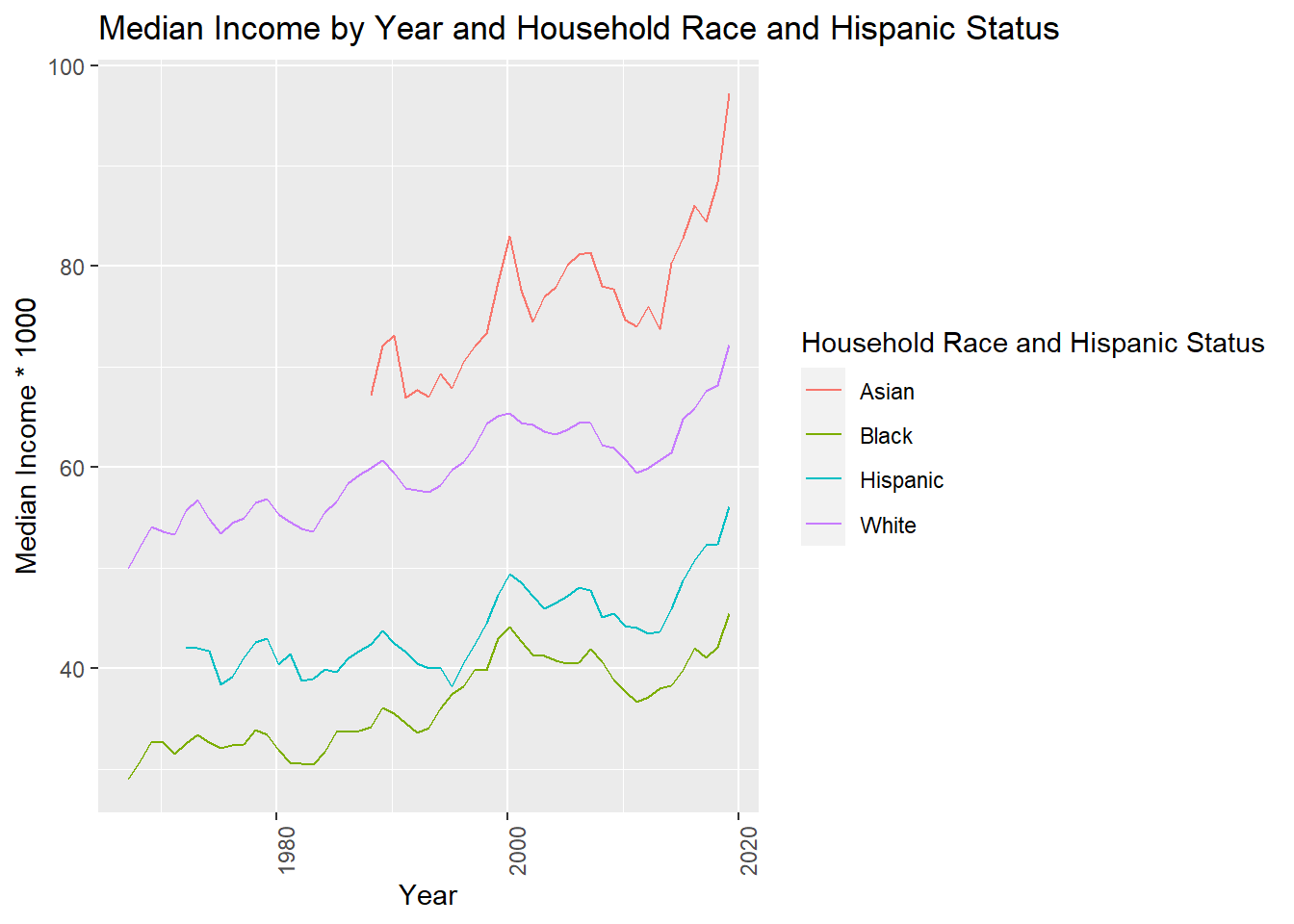

Chunk 4: Time Dependent Visualization (cont)

Weird stuff in the year distribution! Rather than spend a year looking into this, I will limit graph to 2000 forward.

# limit to time period starting in 2000
  usa_hh_tidy_med_income_2020 <-
     usa_hh_tidy_med_income  %>%
     filter(measure_date > '1999-01-01') 
  
  usa_hh_tidy_med_income_2020 %>%
  ggplot( aes(x=measure_date, y=med_income, group=clean_origin, color = clean_origin)) +
    geom_line()+ 
          ggtitle("Median Income 2000-2020, by Year and Household Race and Hispanic Status")+
          labs(y = "Median Income, * $1000)", x = "Year", colour = "Household Race and Hispanic Status")+
          theme(axis.text.x = element_text(angle = 90))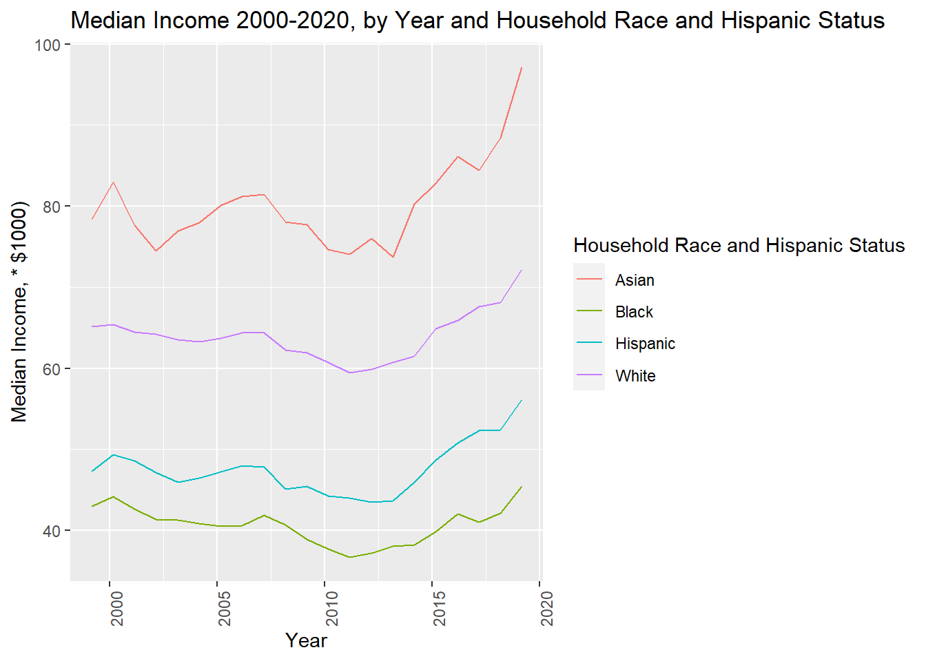

Chunk 5: Visualizing Part-Whole Relationships

I’ll try a couple of things to look at differences income by household race and Hispanic status

A stacked bar char showing percent income by race and Hispanic status over time
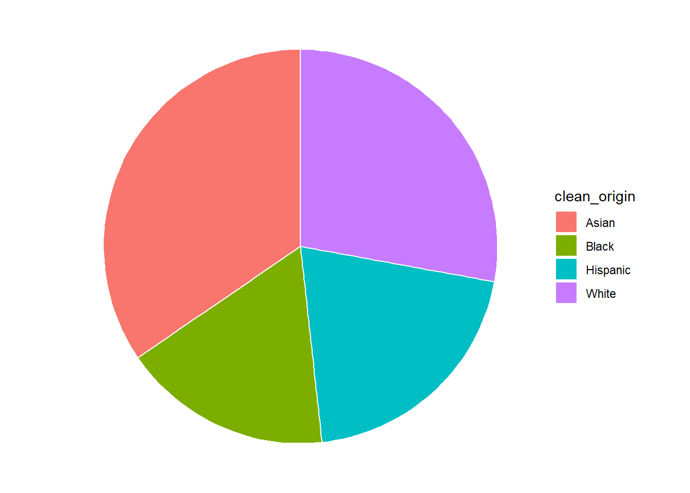
A pie chart based on mean income over all years, 2000 forward

#try a stacked bar
  usa_hh_tidy_pct_med_income_2020 <-
    usa_hh_tidy_med_income_2020 %>%
       group_by(measure_date)%>%
          mutate(perc= med_income/sum(med_income))
  
  ggplot(usa_hh_tidy_pct_med_income_2020, aes(fill=clean_origin, y=perc, x=measure_date)) + 
    geom_bar(position="stack", stat="identity")+ 
          ggtitle("Distribution of Income by Year and Household Race and Hispanic Status")+
          scale_y_continuous(name= "Percent Income", 
                     label = scales::percent)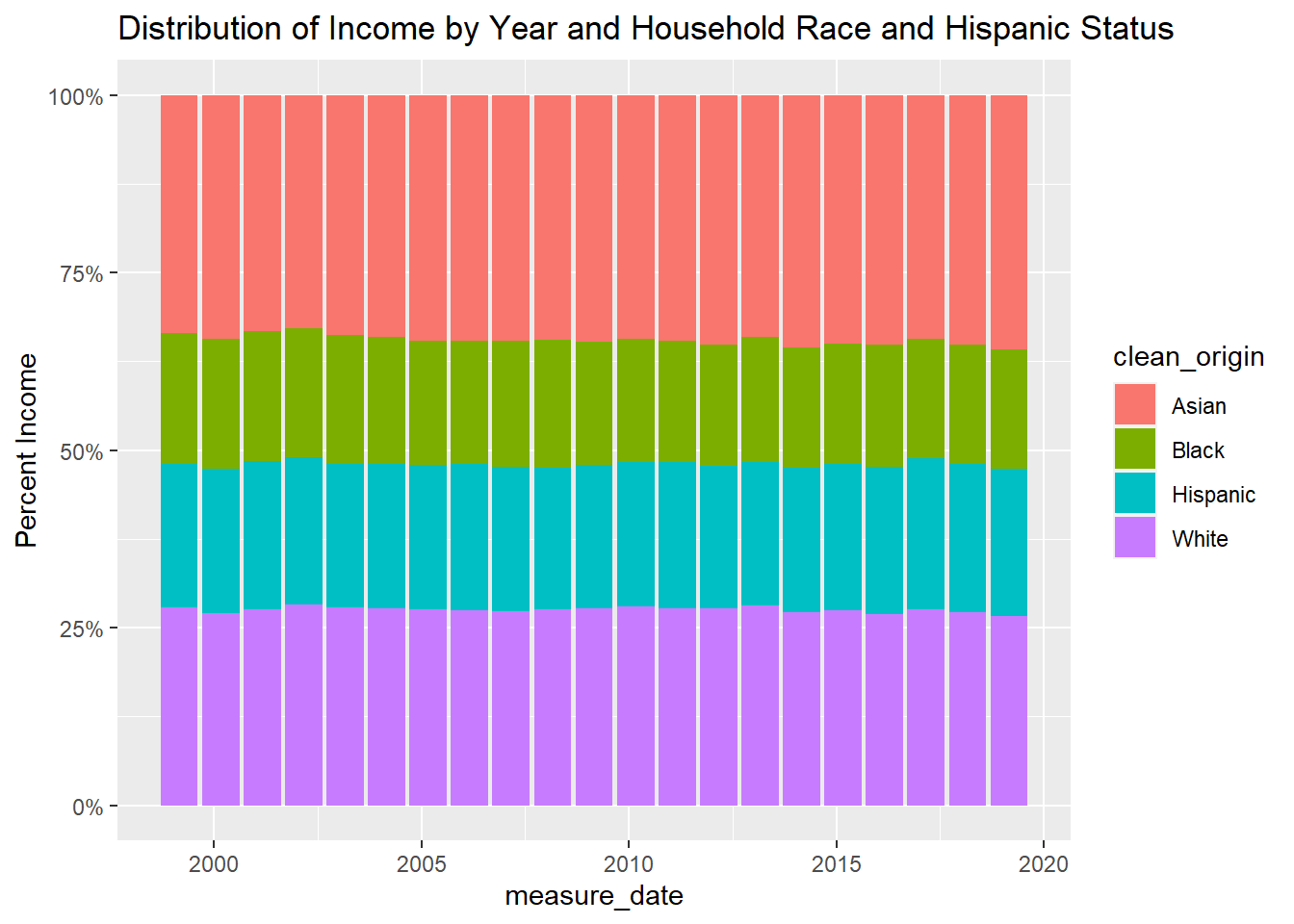

# try a basic pie chart  
 usa_hh_tidy_overall<-
     usa_hh_tidy_g %>%
     filter(measure_date > '1999-01-01' & !clean_origin=="Other") 
  
  usa_hh_tidy_overall_g<-
     usa_hh_tidy_overall %>%
         group_by(clean_origin)%>%
           summarise(med_income = min(med_incomeK)) %>%
              arrange(clean_origin )
  
  ggplot(usa_hh_tidy_overall_g, aes(x="", y=med_income, fill=clean_origin)) +
  geom_bar(stat="identity", width=1, color="white") +
  coord_polar("y", start=0) +
  theme_void()