Challenge 7

Visualizing Multiple Dimensions

library(tidyverse)
library(ggplot2)
library(lubridate)

knitr::opts_chunk$set(echo = TRUE, warning=FALSE, message=FALSE)

Read in data

Read in one (or more) of the following datasets, using the correct R package and command.

• eggs ⭐
• abc_poll ⭐⭐
• australian_marriage ⭐⭐
• hotel_bookings ⭐⭐⭐
• air_bnb ⭐⭐⭐
• us_hh ⭐⭐⭐⭐
• faostat ⭐⭐⭐⭐⭐

data <- read_csv("_data/hotel_bookings.csv")
data

# A tibble: 119,390 × 32
   hotel  is_ca…¹ lead_…² arriv…³ arriv…⁴ arriv…⁵ arriv…⁶ stays…⁷ stays…⁸ adults
   <chr>    <dbl>   <dbl>   <dbl> <chr>     <dbl>   <dbl>   <dbl>   <dbl>  <dbl>
 1 Resor…       0     342    2015 July         27       1       0       0      2
 2 Resor…       0     737    2015 July         27       1       0       0      2
 3 Resor…       0       7    2015 July         27       1       0       1      1
 4 Resor…       0      13    2015 July         27       1       0       1      1
 5 Resor…       0      14    2015 July         27       1       0       2      2
 6 Resor…       0      14    2015 July         27       1       0       2      2
 7 Resor…       0       0    2015 July         27       1       0       2      2
 8 Resor…       0       9    2015 July         27       1       0       2      2
 9 Resor…       1      85    2015 July         27       1       0       3      2
10 Resor…       1      75    2015 July         27       1       0       3      2
# … with 119,380 more rows, 22 more variables: children <dbl>, babies <dbl>,
#   meal <chr>, country <chr>, market_segment <chr>,
#   distribution_channel <chr>, is_repeated_guest <dbl>,
#   previous_cancellations <dbl>, previous_bookings_not_canceled <dbl>,
#   reserved_room_type <chr>, assigned_room_type <chr>, booking_changes <dbl>,
#   deposit_type <chr>, agent <chr>, company <chr>, days_in_waiting_list <dbl>,
#   customer_type <chr>, adr <dbl>, required_car_parking_spaces <dbl>, …

Briefly describe the data

We see that the there are 119,390 rows for hotel entries and 32 columns for information such as reserved room type, deposit type, reservation status, adults (number), country etc. After analyzing the summary() and above commands in R, we can conclude that the data has been collected from 178 countries over a span of 4 years (2014 - 17), going by the reservation dates. We can further conclude that most of the data collected is from 2016 - 17 as the Q1 of reservation status date lies in 2016. It is also clear that there are two kind of hotels (Resort and City Hotel), and 8 types of market segments. From the summary we can also observe that most bookings have adults followed by children and then babies. Further, on an average stay is booked for 2.5 days during week days and around for a day during weekends.

Tidy Data (as needed)

Since we have arrival date, month, year in three different columns we can combine the fields into one single field. The final column is in date/month/year format. Also, the arrival_date_week_number can be dropped as this is not really useful for our analysis.

 data <- data[,-6]

 data<-data%>%
   mutate(date_arrival = str_c(arrival_date_day_of_month,
                               arrival_date_month,
                               arrival_date_year, sep="/"),
          date_arrival = dmy(date_arrival))%>%
  select(-starts_with("arrival"))

Visualization with Multiple Dimensions

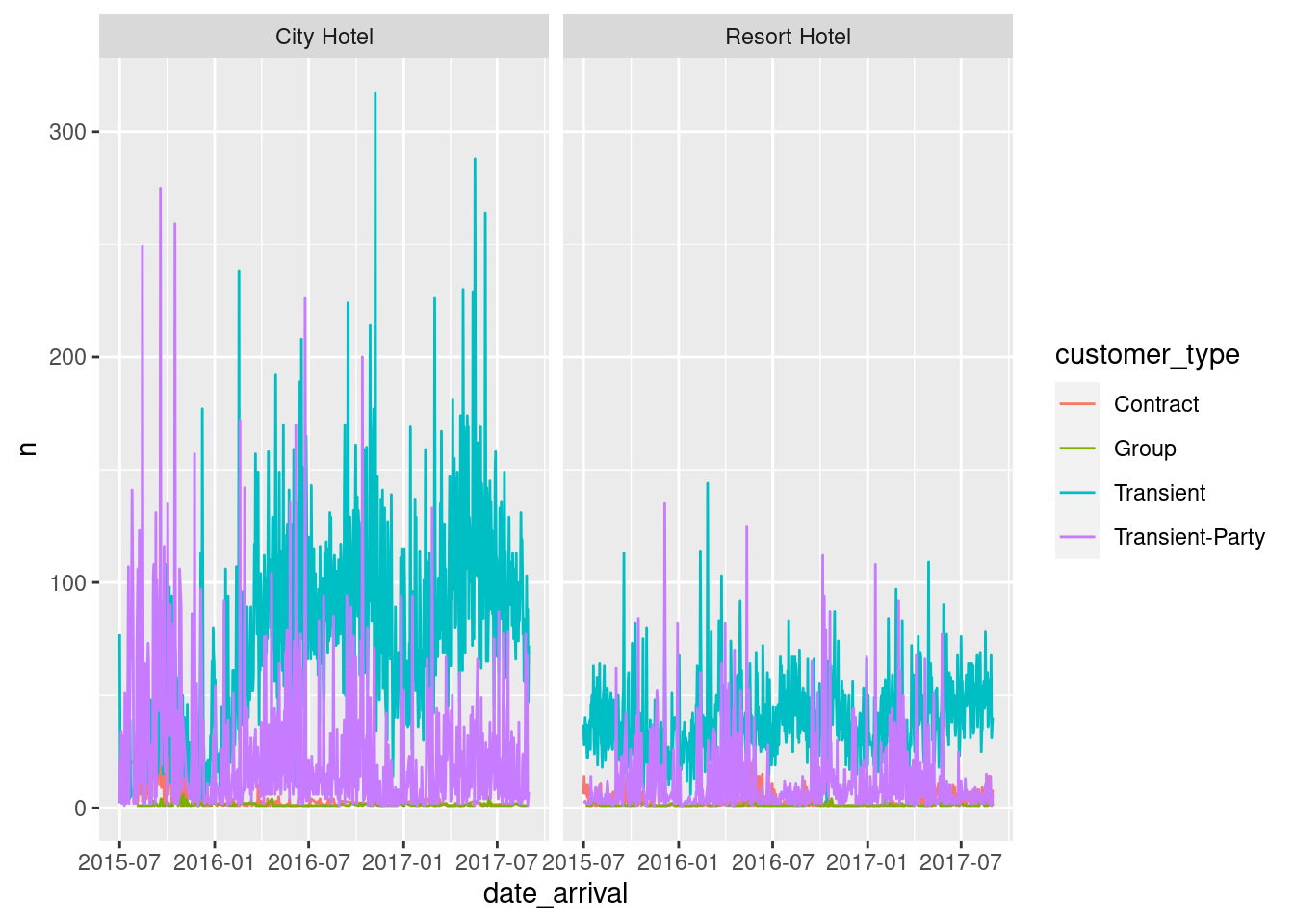
We first group the data by hotel, arrival date, and customer_type. We then plot a multi dimensional graph for number of different types of customers for each type of hotel against arrial dates.

no_of_customers <- data %>%
group_by(hotel, date_arrival, customer_type) %>%
count(hotel, date_arrival, customer_type)
view(no_of_customers)

ggplot(no_of_customers,aes(date_arrival, n, col=customer_type))+
geom_line()+
facet_wrap(vars(hotel))

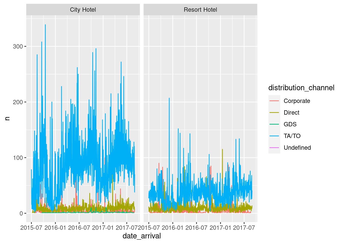
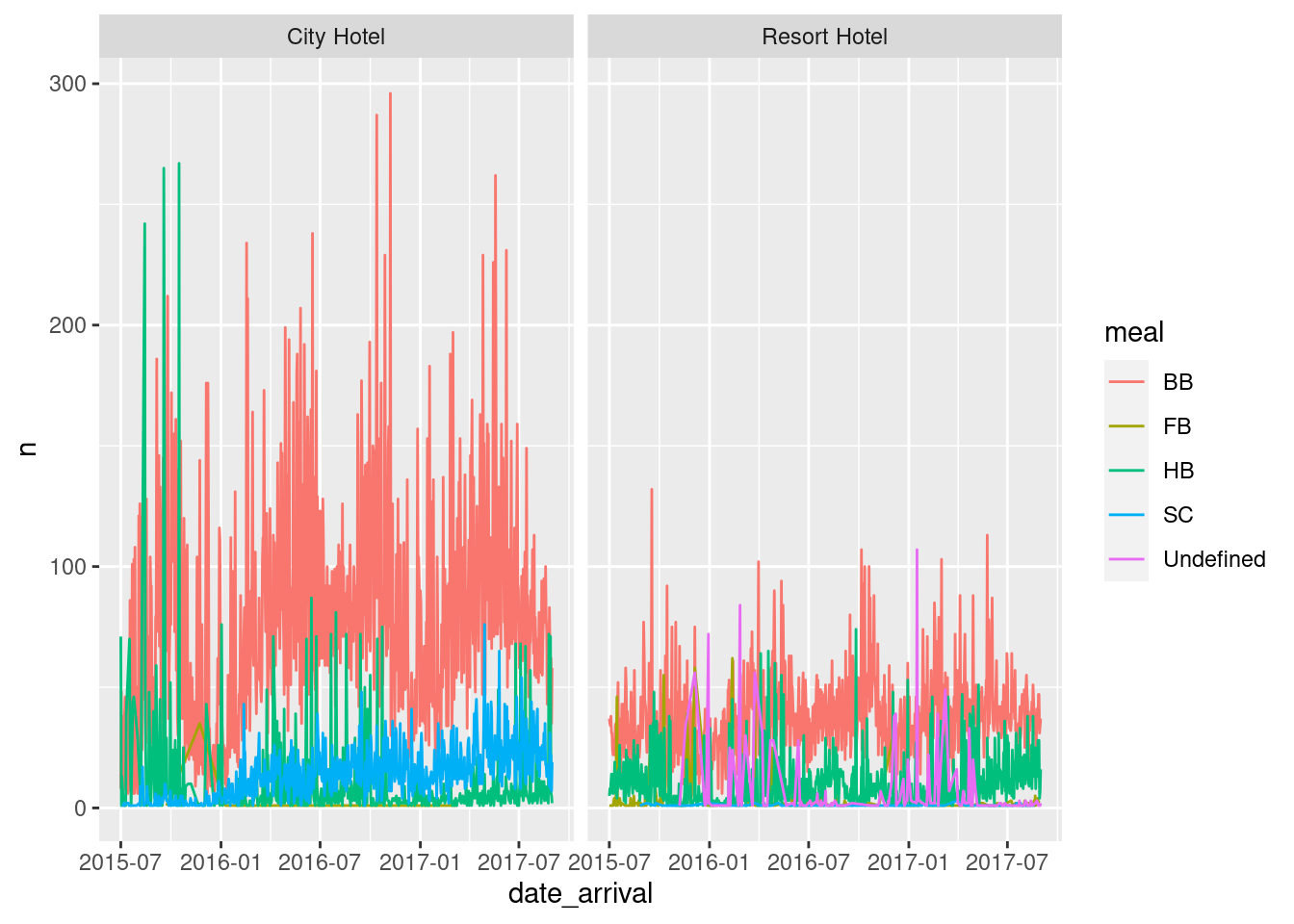
Similar graphs are plotted for distribution channels and meals.

distribution_channels <- data %>%
   group_by(hotel, date_arrival, distribution_channel) %>%
   count(date_arrival, hotel, distribution_channel)
view(distribution_channels)

ggplot(distribution_channels,aes(date_arrival, n, col=distribution_channel))+
geom_line()+
facet_wrap(vars(hotel))

no_of_meals <- data %>%
group_by(hotel, date_arrival, meal) %>%
count(date_arrival, hotel, meal)
view(no_of_meals)

ggplot(no_of_meals,aes(date_arrival, n, col=meal))+
geom_line()+
facet_wrap(vars(hotel))