Challenge 8

Joining Data

library(tidyverse)
library(ggplot2)
library(lubridate)

knitr::opts_chunk$set(echo = TRUE, warning=FALSE, message=FALSE)

Read in data

actors <- read_csv('_data/snl_actors.csv')
casts <- read_csv('_data/snl_casts.csv')
seasons <- read_csv('_data/snl_seasons.csv')

view(actors)
view(casts)
view(seasons)

Briefly describe the data

This data set contains three tables - actors, casts, and seasons of Saturday Night Live show. The actors table contains actors name, type (cast/guest), gender. The casts table contains name, season id, and other information. The seasons table contains season Id, year, and number of episodes. There are a total of 46 seasons from 1975 to 2020.

Join Data

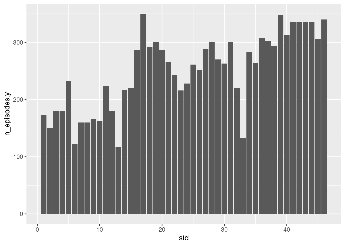
We can first join two tables - casts and seasons by sid. The new table contains information about sid, year, no.of episodes (per season), and number of episodes for each cast member in a season. We can then plot a graph for season number against number of episodes for cast member.

 data <- left_join(seasons, casts, by = "sid" )
 data

# A tibble: 614 × 12
     sid  year first_epi…¹ last_…² n_epi…³ aid   featu…⁴ first…⁵ last_…⁶ updat…⁷
   <dbl> <dbl>       <dbl>   <dbl>   <dbl> <chr> <lgl>     <dbl>   <dbl> <lgl>  
 1     1  1975    19751011  1.98e7      24 Gild… FALSE        NA NA      FALSE  
 2     1  1975    19751011  1.98e7      24 Mich… FALSE        NA  1.98e7 FALSE  
 3     1  1975    19751011  1.98e7      24 Lara… FALSE        NA NA      FALSE  
 4     1  1975    19751011  1.98e7      24 Garr… FALSE        NA NA      FALSE  
 5     1  1975    19751011  1.98e7      24 Jane… FALSE        NA NA      FALSE  
 6     1  1975    19751011  1.98e7      24 Geor… FALSE        NA  1.98e7 FALSE  
 7     1  1975    19751011  1.98e7      24 Chev… FALSE        NA NA      TRUE   
 8     1  1975    19751011  1.98e7      24 John… FALSE        NA NA      FALSE  
 9     1  1975    19751011  1.98e7      24 Dan … FALSE        NA NA      FALSE  
10     2  1976    19760918  1.98e7      22 Gild… FALSE        NA NA      FALSE  
# … with 604 more rows, 2 more variables: n_episodes.y <dbl>,
#   season_fraction <dbl>, and abbreviated variable names ¹​first_epid.x,
#   ²​last_epid.x, ³​n_episodes.x, ⁴​featured, ⁵​first_epid.y, ⁶​last_epid.y,
#   ⁷​update_anchor

 data %>%
 ggplot(aes(x = sid, y = n_episodes.y)) +
 geom_bar(stat = "identity") 

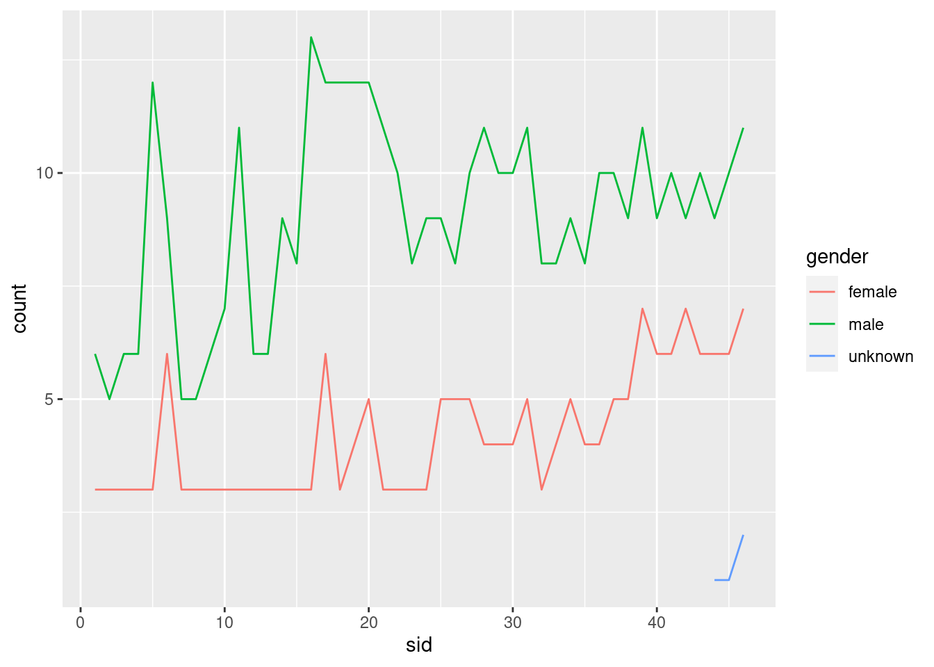
For another plot, we can then merge actors and casts by aid. This table can later be joined with seasons table by sid. Below, we plot another graph to depict the number of male and female in each season of SNL.

actors_casts <- merge(actors, casts, by = 'aid')

actors_casts_gender <- actors_casts %>%
merge(seasons, by = 'sid') %>%
group_by(sid, year, gender) %>%
count(sid, gender)

actors_casts_gender %>%
ggplot(aes(sid, n, col = gender)) +
geom_line() +
ylab("count")