Challenge 9

Creating a function

library(tidyverse)
library(ggplot2)
library(dplyr)

knitr::opts_chunk$set(echo = TRUE, warning=FALSE, message=FALSE)

Challenge Overview

Today’s challenge is simple. Create a function, and use it to perform a data analysis / cleaning / visualization task:

Examples of such functions are: 1) A function that reads in and cleans a dataset.
2) A function that computes summary statistics (e.g., computes the z score for a variable).
3) A function that plots a histogram.

That’s it!

Function to read and clean a dataset

This function reads in a csv and removes the N/A columns in the file

read_and_clean_csv <- function(x) {
  data <- read_csv(x)
  data <- data %>% select_if(~ !any(is.na(.)))
  return(data)
} 

Running the function on the dataset hotel_bookings.csv

data <- read_and_clean_csv("_data/hotel_bookings.csv")
head(data)

# A tibble: 6 × 31
  hotel   is_ca…¹ lead_…² arriv…³ arriv…⁴ arriv…⁵ arriv…⁶ stays…⁷ stays…⁸ adults
  <chr>     <dbl>   <dbl>   <dbl> <chr>     <dbl>   <dbl>   <dbl>   <dbl>  <dbl>
1 Resort…       0     342    2015 July         27       1       0       0      2
2 Resort…       0     737    2015 July         27       1       0       0      2
3 Resort…       0       7    2015 July         27       1       0       1      1
4 Resort…       0      13    2015 July         27       1       0       1      1
5 Resort…       0      14    2015 July         27       1       0       2      2
6 Resort…       0      14    2015 July         27       1       0       2      2
# … with 21 more variables: babies <dbl>, meal <chr>, country <chr>,
#   market_segment <chr>, distribution_channel <chr>, is_repeated_guest <dbl>,
#   previous_cancellations <dbl>, previous_bookings_not_canceled <dbl>,
#   reserved_room_type <chr>, assigned_room_type <chr>, booking_changes <dbl>,
#   deposit_type <chr>, agent <chr>, company <chr>, days_in_waiting_list <dbl>,
#   customer_type <chr>, adr <dbl>, required_car_parking_spaces <dbl>,
#   total_of_special_requests <dbl>, reservation_status <chr>, …

Function to compute statistics (z-score)

z-score = (x - mean) / std_dev

z_score <- function(col) {
  output <- (col - mean(col)) / sd(col)
  return(output)
}

Evaluating Z-Score for a column in hotel_bookings.csv

z_score_output <- z_score(data$stays_in_week_nights)
head(z_score_output)

[1] -1.3102344 -1.3102344 -0.7862039 -0.7862039 -0.2621733 -0.2621733

Function that plots a histogram

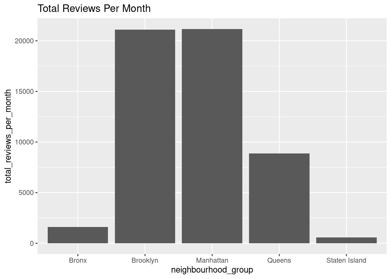
plot_histogram <- function(input_path) {
  tidy_data <- read_csv(input_path)
  tidy_data <- tidy_data %>% replace_na(list(reviews_per_month = 0))
  df_agg = tidy_data %>% group_by(neighbourhood_group)  %>%
                    summarise(total_reviews_per_month = sum(reviews_per_month),
                              .groups = 'drop')
  head(df_agg)
  ggplot(data=df_agg, aes(x=neighbourhood_group, y=total_reviews_per_month)) +
  geom_bar(stat="identity") + labs(title = "Total Reviews Per Month")
}

plot_histogram("_data/AB_NYC_2019.csv")