Challenge 6

Visualizing Time and Relationships

library(tidyverse)
library(ggplot2)
library(lubridate)

knitr::opts_chunk$set(echo = TRUE, warning=FALSE, message=FALSE)

Challenge Overview

Today’s challenge is to:

1. read in a data set, and describe the data set using both words and any supporting information (e.g., tables, etc)
2. tidy data (as needed, including sanity checks)
3. mutate variables as needed (including sanity checks)
4. create at least one graph including time (evolution)

• try to make them “publication” ready (optional)
• Explain why you choose the specific graph type

5. Create at least one graph depicting part-whole or flow relationships

• try to make them “publication” ready (optional)
• Explain why you choose the specific graph type

R Graph Gallery is a good starting point for thinking about what information is conveyed in standard graph types, and includes example R code.

(be sure to only include the category tags for the data you use!)

Read in data

Read in one (or more) of the following datasets, using the correct R package and command.

• debt ⭐
• fed_rate ⭐⭐
• abc_poll ⭐⭐⭐
• usa_hh ⭐⭐⭐
• hotel_bookings ⭐⭐⭐⭐
• air_bnb ⭐⭐⭐⭐⭐

hotel_bookings= read_csv("../posts/_data/hotel_bookings.csv")
head(hotel_bookings)

# A tibble: 6 × 32
  hotel   is_ca…¹ lead_…² arriv…³ arriv…⁴ arriv…⁵ arriv…⁶ stays…⁷ stays…⁸ adults
  <chr>     <dbl>   <dbl>   <dbl> <chr>     <dbl>   <dbl>   <dbl>   <dbl>  <dbl>
1 Resort…       0     342    2015 July         27       1       0       0      2
2 Resort…       0     737    2015 July         27       1       0       0      2
3 Resort…       0       7    2015 July         27       1       0       1      1
4 Resort…       0      13    2015 July         27       1       0       1      1
5 Resort…       0      14    2015 July         27       1       0       2      2
6 Resort…       0      14    2015 July         27       1       0       2      2
# … with 22 more variables: children <dbl>, babies <dbl>, meal <chr>,
#   country <chr>, market_segment <chr>, distribution_channel <chr>,
#   is_repeated_guest <dbl>, previous_cancellations <dbl>,
#   previous_bookings_not_canceled <dbl>, reserved_room_type <chr>,
#   assigned_room_type <chr>, booking_changes <dbl>, deposit_type <chr>,
#   agent <chr>, company <chr>, days_in_waiting_list <dbl>,
#   customer_type <chr>, adr <dbl>, required_car_parking_spaces <dbl>, …

Briefly describe the data

For this assignment I’m choosing to work with the hotels data because I’ve worked with it on a previous challenge and am fairly comfortable with it. ## Tidy Data (as needed)

Is your data already tidy, or is there work to be done? Be sure to anticipate your end result to provide a sanity check. Are there any variables that require mutation to be usable in your analysis stream? For example, do you need to calculate new values in order to graph them? Can string values be represented numerically? Do you need to turn any variables into factors and reorder for ease of graphics and visualization?

Document your work here.

tidy_bookings <- 
  hotel_bookings %>%
      mutate(arrival=str_c(arrival_date_day_of_month, arrival_date_month,arrival_date_year, sep="/"), arrival=dmy(arrival)) 

tidy_bookings = select(tidy_bookings, select = -starts_with("arrival_date"))

Here we do the same process to the data as we did earlier- organize those date variables into one standard date, instead of being in 3 separate columns (day, month, year). This makes the data tidier, simpler, and more accessible.

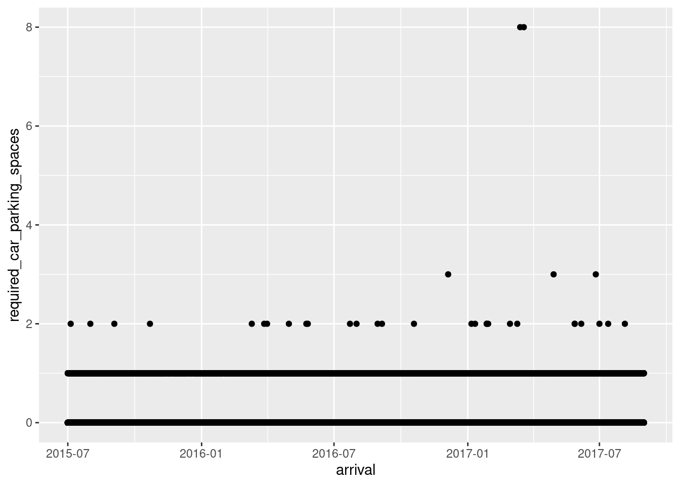
Now we want to be able to take a portion of the time we have data listed under, and use it gain some insight. As a pseudo hotel manager, lets use our knowledge of the bookings CSV to try to see if we can set up reserved parking spaces for non-employees, whenever guests may need- lets try to look at how the demand for parking spaces fluctuates over time;

ggplot(tidy_bookings, aes(arrival, required_car_parking_spaces)) + (geom_point()) 

Not very insightful! our date blocks (6 months) are too wide, and we don’t want to look at three years worth of data anyway. Lets narrow down our range and decrease block size, so we can get a better look.

Time Dependent Visualization

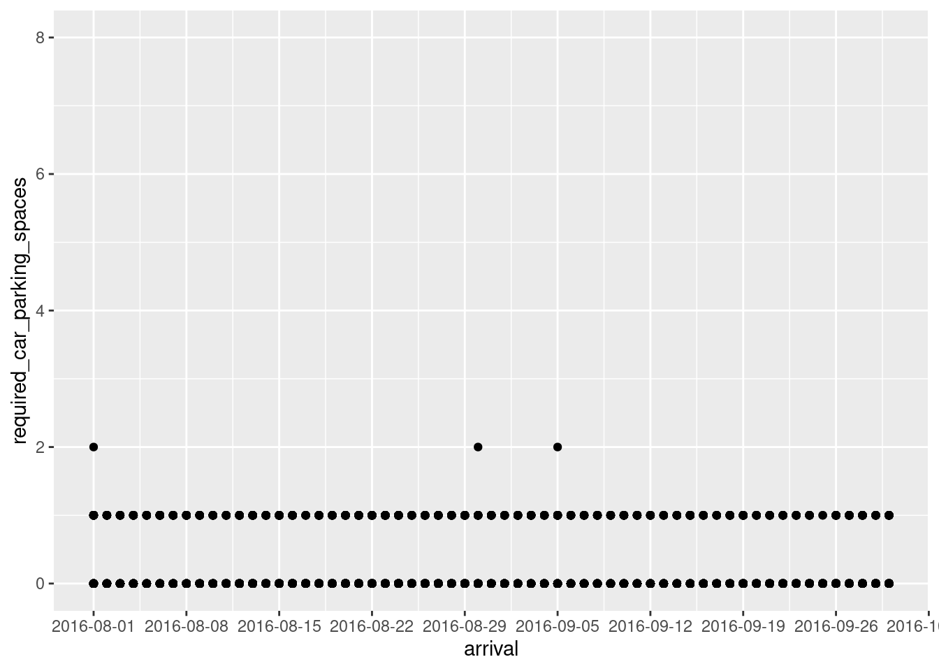
Here, we narrow down the date fields to just the months of August and September in the year 2016. We want to know how many parking spaces we’ll need to have reserved for our guests at all times, so by splitting this time up into weeks and putting number of spaces required on the y-axis, we can keep track of how many spaces we need each week of that two month period.

ggplot(tidy_bookings, aes(arrival, required_car_parking_spaces)) + (geom_point()) +
  scale_x_date(date_breaks = '1 week',
  limits = as.Date(c('2016-8-1', '2016-9-30')))