Challenge 9 Yoshita Varma

Creating a function

library(tidyverse)
library(ggplot2)

knitr::opts_chunk$set(echo = TRUE, warning=FALSE, message=FALSE)

Challenge Overview

Today’s challenge is simple. Create a function, and use it to perform a data analysis / cleaning / visualization task:

Examples of such functions are: 1) A function that reads in and cleans a dataset.
2) A function that computes summary statistics (e.g., computes the z score for a variable).
3) A function that plots a histogram.

That’s it!

A function that reads in and cleans a dataset.

func_read_clean <- function(x) {
  data <- read_csv(x)
  data <- data %>% select_if(~ !any(is.na(.)))
  return(data)
} 

Reading hotel booking data as I am familiar with it.

hotel_booking <- func_read_clean("_data/hotel_bookings.csv")
hotel_booking

# A tibble: 119,390 × 31
   hotel  is_ca…¹ lead_…² arriv…³ arriv…⁴ arriv…⁵ arriv…⁶ stays…⁷ stays…⁸ adults
   <chr>    <dbl>   <dbl>   <dbl> <chr>     <dbl>   <dbl>   <dbl>   <dbl>  <dbl>
 1 Resor…       0     342    2015 July         27       1       0       0      2
 2 Resor…       0     737    2015 July         27       1       0       0      2
 3 Resor…       0       7    2015 July         27       1       0       1      1
 4 Resor…       0      13    2015 July         27       1       0       1      1
 5 Resor…       0      14    2015 July         27       1       0       2      2
 6 Resor…       0      14    2015 July         27       1       0       2      2
 7 Resor…       0       0    2015 July         27       1       0       2      2
 8 Resor…       0       9    2015 July         27       1       0       2      2
 9 Resor…       1      85    2015 July         27       1       0       3      2
10 Resor…       1      75    2015 July         27       1       0       3      2
# … with 119,380 more rows, 21 more variables: babies <dbl>, meal <chr>,
#   country <chr>, market_segment <chr>, distribution_channel <chr>,
#   is_repeated_guest <dbl>, previous_cancellations <dbl>,
#   previous_bookings_not_canceled <dbl>, reserved_room_type <chr>,
#   assigned_room_type <chr>, booking_changes <dbl>, deposit_type <chr>,
#   agent <chr>, company <chr>, days_in_waiting_list <dbl>,
#   customer_type <chr>, adr <dbl>, required_car_parking_spaces <dbl>, …

A function that computes summary statistics (e.g., computes the z score for a variable).

statistics <- function(x){
  stat <- tibble(
    mean=mean(x),
    median=median(x),
    sd=sd(x)
  )
  return(stat)
}
statistics(hotel_booking$stays_in_week_nights)

# A tibble: 1 × 3
   mean median    sd
  <dbl>  <dbl> <dbl>
1  2.50      2  1.91

Printing stats of stays_in_week_nights.

A function that plots a histogram.

histogram <- function(data_read){
  HotelBookings_csv_mutate <- data_read %>% 
  mutate(arrival_date = str_c(arrival_date_year, 
                              arrival_date_month, arrival_date_day_of_month, sep="/"),
         arrival_date = lubridate::ymd(arrival_date)) %>% 
  select(-c(arrival_date_year,arrival_date_month, arrival_date_day_of_month))

  
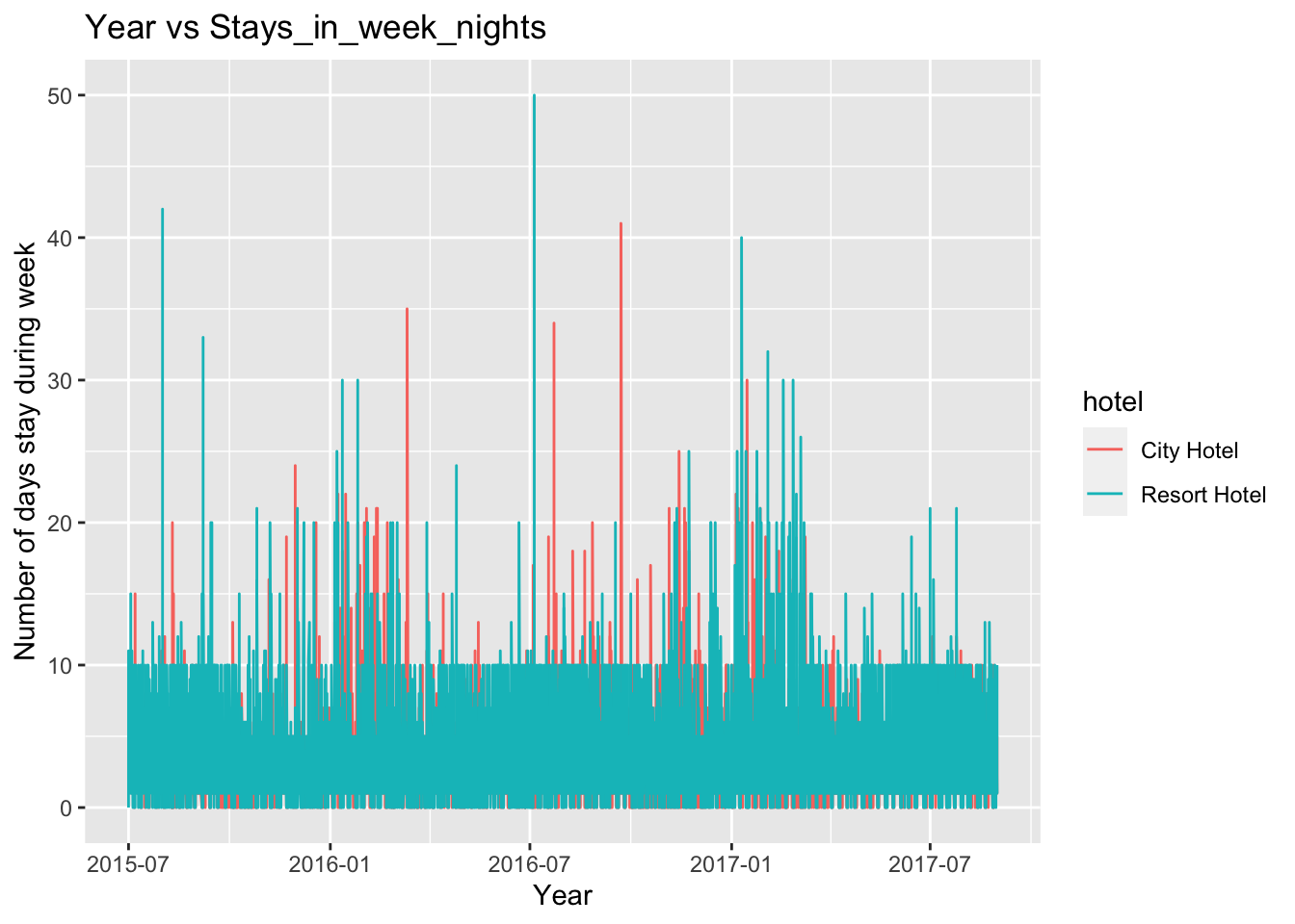
ggplot(HotelBookings_csv_mutate, aes(x=arrival_date, y= stays_in_week_nights, color = `hotel`)) + 
  geom_line() + 
  xlab("Year") + 
  ylab("Number of days stay during week") + 
  ggtitle("Year vs Stays_in_week_nights")
}

histogram(hotel_booking)

This shows some might book a hotel instead of renting a place. One common thing observed is the spike in the start of the year.