Homework 1

Code

knitr::opts_chunk$set(echo = TRUE)

Loading in packages:

Code

library(readr)
library(ggplot2)
library(dplyr)

Attaching package: 'dplyr'

The following objects are masked from 'package:stats':

    filter, lag

The following objects are masked from 'package:base':

    intersect, setdiff, setequal, union

Code

library(readxl)

Reading in Data:

Code

df <- read_excel('_data/LungCapData.xls')
df

# A tibble: 725 × 6
   LungCap   Age Height Smoke Gender Caesarean
     <dbl> <dbl>  <dbl> <chr> <chr>  <chr>    
 1    6.48     6   62.1 no    male   no       
 2   10.1     18   74.7 yes   female no       
 3    9.55    16   69.7 no    female yes      
 4   11.1     14   71   no    male   no       
 5    4.8      5   56.9 no    male   no       
 6    6.22    11   58.7 no    female no       
 7    4.95     8   63.3 no    male   yes      
 8    7.32    11   70.4 no    male   no       
 9    8.88    15   70.5 no    male   no       
10    6.8     11   59.2 no    male   no       
# … with 715 more rows

1(a) Distribution of LungCap:

Code

hist(df$LungCap)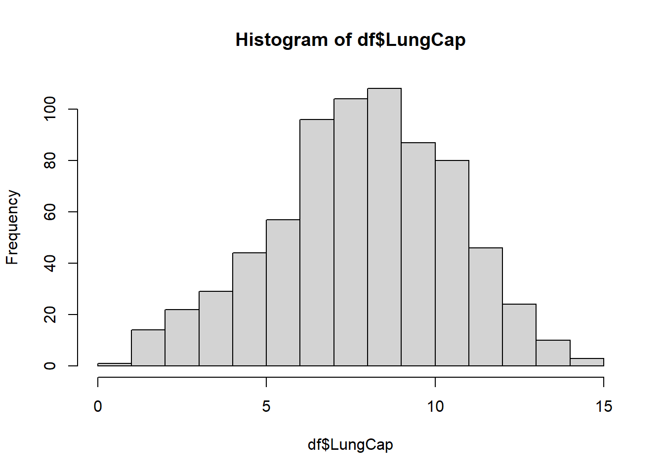

The distribution appears to be very similar to a normal distribution, according to the histogram.

1(b)

The boxplots below show the probability distributions grouped by Gender.

Code

boxplot(LungCap~Gender, data=df)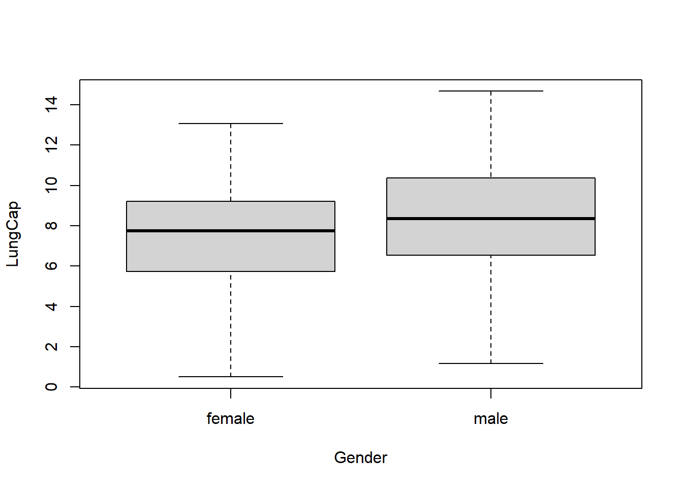

Looks like males have a slightly higher lung capacity than females.

1 (c)

Code

df %>%
  group_by(Smoke) %>%
  summarize(Mean = mean(LungCap))

# A tibble: 2 × 2
  Smoke  Mean
  <chr> <dbl>
1 no     7.77
2 yes    8.65

Surprisingly, the mean lung capacity is higher for smokers than it is for non-smokers.

1 (d)

Code

# convert Age to categorical variable.
df <- mutate(df, AgeGroup = case_when(Age <= 13 ~ "13 and lower", Age == 14 | Age == 15 ~ "14-15", Age == 16 | Age == 17 ~ "16-17", Age >= 18 ~ "18 and above"))
arrange(df, Age)

# A tibble: 725 × 7
   LungCap   Age Height Smoke Gender Caesarean AgeGroup    
     <dbl> <dbl>  <dbl> <chr> <chr>  <chr>     <chr>       
 1   5.88      3   55.9 no    male   no        13 and lower
 2   0.507     3   51.6 no    female yes       13 and lower
 3   1.18      3   51.9 no    male   no        13 and lower
 4   4.7       3   52.7 no    male   no        13 and lower
 5   5.48      3   52.9 no    male   no        13 and lower
 6   1.02      3   47   no    female no        13 and lower
 7   2         3   51   no    female no        13 and lower
 8   1.68      3   51.9 no    male   no        13 and lower
 9   4.08      3   53.6 no    male   yes       13 and lower
10   1.45      3   45.3 no    female no        13 and lower
# … with 715 more rows

Code

# construct histogram.
ggplot(df, aes(x = LungCap)) +
  geom_histogram() +
  facet_grid(AgeGroup~Smoke)

`stat_bin()` using `bins = 30`. Pick better value with `binwidth`.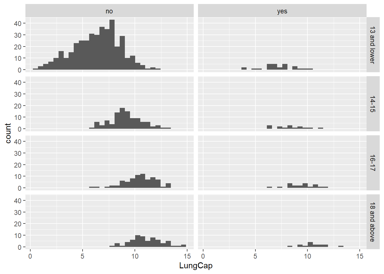

Majority seem to be non-smokers, and looks like non-smokers seem to have higher lung capacity.

1 (e)

Code

class(df$AgeGroup)

[1] "character"

Code

df$AgeGroup <- as.factor(df$AgeGroup) #converting to factor

# construct table.
df %>% select(Smoke, LungCap, AgeGroup) %>% group_by(AgeGroup, Smoke) %>% summarise(mean(LungCap))

`summarise()` has grouped output by 'AgeGroup'. You can override using the
`.groups` argument.

# A tibble: 8 × 3
# Groups:   AgeGroup [4]
  AgeGroup     Smoke `mean(LungCap)`
  <fct>        <chr>           <dbl>
1 13 and lower no               6.36
2 13 and lower yes              7.20
3 14-15        no               9.14
4 14-15        yes              8.39
5 16-17        no              10.5 
6 16-17        yes              9.38
7 18 and above no              11.1 
8 18 and above yes             10.5 

The mean lung capacity for smokers aged 13 and under is greater than that of non-smokers in the same age group which is different from expectation. Non-smokers have higher mean lung capacity for ages 14-15, 16-17 and 18 and above. Either there may be an error or extreme outlier in the data for smokers aged 13 and under.

1 (f)

Code

cor(df$LungCap,df$Age)

[1] 0.8196749

Code

cov(df$LungCap,df$Age)

[1] 8.738289

Lung capacity and age have a high positive correlation of 0.82, meaning that as age increases, lung capacity also does. The covariance is a little more challenging to interpret; the positive number indicates a positive association between lung capacity and age, but because covariance varies from negative infinity to infinity, it is difficult to judge the strength of the relationship. In most situations, I would choose to employ correlation.

2

Code

df1 <- c(0:4)
Inmate_count <- c(128, 434, 160, 64, 24)
IP<- data_frame(df1, Inmate_count)

Warning: `data_frame()` was deprecated in tibble 1.1.0.
ℹ Please use `tibble()` instead.

2(a)

Code

IP <- mutate(IP, Probability = Inmate_count/sum(Inmate_count))
IP

# A tibble: 5 × 3
    df1 Inmate_count Probability
  <int>        <dbl>       <dbl>
1     0          128      0.158 
2     1          434      0.536 
3     2          160      0.198 
4     3           64      0.0790
5     4           24      0.0296

Code

IP %>%
  filter(df1 == 2) %>%
  select(Probability)

# A tibble: 1 × 1
  Probability
        <dbl>
1       0.198

The probability is about 19.75%.

(b)

Code

df2 <- IP %>%
  filter(df1 < 2)
sum(df2$Probability)

[1] 0.6938272

The probability that a randomly selected inmate has fewer than 2 prior convictions is 0.6938272

2(c)

Code

df3 <- IP %>%
  filter(df1 <= 2)
sum(df3$Probability)

[1] 0.891358

The probability that a randomly selected inmate has 2 or fewer prior convictions is 0.891358.

2(d)

Code

df4 <- IP %>%
  filter(df1 > 2)
sum(df4$Probability)

[1] 0.108642

The probability that a randomly selected inmate has more than 2 prior convictions is 0.108642.

2(e)

Code

IP <- mutate(IP, X = df1*Probability)
expectedvalue<- sum(IP$X)
expectedvalue

[1] 1.28642

The expected value for the number of prior convictions is 1.2864198. We can round this to 1.

2(f)

Code

var1 <-sum(((IP$df1-expectedvalue)^2)*IP$Probability)
var1

[1] 0.8562353

Code

sqrt(var1)

[1] 0.9253298

The variance and the standard deviation for prior convictions are 0.8562353 and 0.9253298 respectively.