Final Project Part 2

finalpart2

Author

Emma Rasmussen

Published

November 11, 2022

knitr::opts_chunk$set(echo = TRUE, warning=FALSE, message=FALSE)

library(readxl)
library(tidyverse)
library(ggplot2)
library(dplyr)
library(stringr)
library(googlesheets4)
library(plotly)

Research Question

Does political partisanship correlate with COVID-19 death rates?

Introduction

The COVID-19 pandemic became a political matter. Behaviors associated with COVID-19 prevention were adopted on partisan lines (masking, social distancing, and vaccine uptake). Early in the pandemic, mask mandates were protested in some communities. My research question is have these behaviors affected COVID-19 death rates along partisan lines? If so, public health interventions could target communities that may be higher risk for COVID-19 deaths based on political partisanship.

For this analysis I used cumulative COVID-19 death toll as opposed to infection rates as infection rates are constantly changing over time. Other studies have looked at infection rates on partisan lines over waves of the pandemic, see this study from the Pew Research Center (Jones 2022)). I measured partisanship using 2016 county-level election results (% voting for Trump). My research is looking to see if (county-level) Trump support correlates with COVID-19 death rates. The unit of analysis for this study was U.S. counties.

I also control for age (percent population over 65), income (median household income in 2020), urbanization (Urban-Rural Continuum Code), and policy (2020 governor dummy variable).

Hypothesis

While I came up with this research idea on my own, other organizations such as NPR (Wood and Brumfiel 2021) and the Pew Research Center (Jones 2022) have already tested this and found a significant correlation in Trump support and COVID-19 death and infection rates. For this project, I will use more recent data and include additional control variables that were not accounted for in these previous studies.

H0: B1 is zero. There is no correlation between political partisanship and COVID-19 death rates. Ha: B1 is not zero. There is a correlation between partisanship and COVID-19 death rates.

Variables

Political Partisanship

For this project, I measured partisanship as percentage of the county that voted for Trump in the 2016 election against Clinton. I did not use 2020 election results in case counties “flipped” support as a result of COVID-19. Below I tidied the data, filtering out only 2016 election results, created a variable: percent voting for Trump in 2016, and selected the percent_trump and FIPS Code variables to use in the analysis.

The data used for this variable came from the MIT Election Data and Science Lab (2021).

gs4_deauth()

#2016 election df

votedf<-read_sheet("https://docs.google.com/spreadsheets/d/1fmxoA_bibvsxsvgRdVPCgMA7DkmJNZfxiWgLgCLcsOY/edit#gid=937778872")

votedf$county_fips <- as.character(votedf$county_fips)
votedf<-mutate(votedf, county_fipsNEW=str_pad(votedf$county_fips, 5, pad = "0"))
votedf<-votedf %>% 
  filter(year==2016, candidate=="DONALD TRUMP")
  votedf$percent_trump <-votedf$candidatevotes/votedf$totalvotes
  
votedf<- select(votedf, county_fipsNEW, percent_trump)
head(votedf)

# A tibble: 6 × 2
  county_fipsNEW percent_trump
  <chr>                  <dbl>
1 01001                  0.728
2 01003                  0.765
3 01005                  0.521
4 01007                  0.764
5 01009                  0.893
6 01011                  0.242

COVID-19 Cumulative Death Rate

This data comes from USAFacts.org. Their collection methods are thoroughly described on their website (see USA Facts 2022 in References). Originally I planned on using CDC/NIH data, however they only had data for a little over 1,000 counties, compared to USAFacts which had data for over 3,000. USAFacts compiles their data from CDC, but also town, county, and state leading to a larger number of observations in their dataset.

Cumulative county-level death toll is taken as of March 19, 2022, when many states stopped regularly reporting COVID-19 deaths (and beginning late in January 2020) (USA Facts 2022).

coviddf_2<-read_sheet("https://docs.google.com/spreadsheets/d/1ZKa3sg_UdtyX5z0OGGVZN6nuqcC_OKWcsOjm1ZHNjQY/edit#gid=716391091")

#adding leading 0 back to fips
coviddf_2<-mutate(coviddf_2, county_fipsNEW=str_pad(coviddf_2$"countyFIPS", 5, pad = "0"))

#selecting march 19, 2022, the day before the first day of spring in 2022, when many states stopped/slowed reporting (USA Facts)
coviddf_2<-select(coviddf_2, county_fipsNEW, "County Name", State, "2022-03-19")
coviddf_2<-rename(coviddf_2, "covid_deaths" = "2022-03-19")

Control: Age

Because age correlates with political party and older Americans (over 65) were disproportionately more likely to die as a result of COVID-19, this is included in the analysis as a control. According to an article from the Mayo Clinic Website, 81% of COVID-19 deaths occured in individuals 65 or over (Mayo Clinic Staff 2022). Previous studies have controlled for age as well (Brumfiel and Wood 2021). I controlled for age by creating the variable: percent of the county’s population over 65 years of age.

#age df

#Please see pdf of code tidying I did to make df into a manageable size for google sheets

age<- read_sheet("https://docs.google.com/spreadsheets/d/1EysREWJ61NCSYyiYH8-2pmZC_TnuLTgqa8Lz5ZpsPZ4/edit#gid=271068707")
head(age)

# A tibble: 6 × 6
  STNAME  CTYNAME        county_fipsNEW tot_pop over65 over65_pct         
  <chr>   <chr>          <chr>          <chr>   <chr>  <chr>              
1 Alabama Autauga County 01001          55869   8924   0.1597307988329843 
2 Alabama Baldwin County 01003          223234  46830  0.20977987224168362
3 Alabama Barbour County 01005          24686   4861   0.19691323017094708
4 Alabama Bibb County    01007          22394   3733   0.16669643654550326
5 Alabama Blount County  01009          57826   10814  0.18700930377338915
6 Alabama Bullock County 01011          10101   1711   0.1693891693891694

Control: Policy Dummy Variable

This variable (2020 governor party) attempts to control for local and state policy such as mask mandates, stay-at-home orders, and vaccine requirements to attend large events that contribute to COVID-19 death and infection rates. This data set was created from a table of current U.S. governors and their political party on Ballotpedia.org (2022). I adjusted a couple observations when governors had been elected more recently than March 11, when the WHO declared COVID-19 a global pandemic. This data represents the political party of state governors as of March 11, 2020.

#Governor/policy df

#reading in gov dummy variable: whoever was in office March 11, 2020 (when WHO declared covid-19 a global pandemic)

gov2020<-read_sheet("https://docs.google.com/spreadsheets/d/1-pToTikvnXl1-lT-xazjoxX0sOCwOH5-7Bl8vJqu9Tk/edit#gid=0")

gov2020$Office<-str_remove(gov2020$Office, "Governor of ")
gov2020<-rename(gov2020, "STNAME" = Office)
gov2020<-select(gov2020, STNAME, Name, Party)
head(gov2020)

# A tibble: 6 × 3
  STNAME         Name                 Party     
  <chr>          <chr>                <chr>     
1 Alabama        Kay Ivey             Republican
2 Alaska         Mike Dunleavy        Republican
3 American Samoa Lemanu Palepoi Mauga Democratic
4 Arizona        Doug Ducey           Republican
5 Arkansas       Asa Hutchinson       Republican
6 California     Gavin Newsom         Democratic

Control: Income

Median household income by county in 2020 is taken from this dataset, from the Economic Research Service at United States Department of Agriculture (2022). Income likely correlates with both political affiliation and COVID-19 death rates (access to medical care, preventative treatment etc), which is why it is included in the analysis.

Control: Rural-Urban Continuum Code

This is also taken from the Economic Research Service/USDA dataset. According to the USDA, the 2013 rural-urban continuum code is a “classification scheme that distinguishes metropolitan counties by the population size of their metro area, and nonmetropolitan counties by degree of urbanization and adjacency to a metro area”. In my opinion, this makes more sense to include than a simple calculation of population density, because it takes into account cities/ how close people settle to cities rather than just population divided by land area. (For instance, a large county, land-wise, may have a majority of the population in a large city, however this could still result in a fairly small population density depending on land area). The Rural Urban Continuum code is on an integer scale from 1 to 9, where 1 represents the most urban/metro counties, and 9 represents the most rural counties.

Generally speaking, more rural counties tend to favor Trump while more metropolitan areas tend to be more democratic. At the same time, one would expect that more densely populated areas/ people living closer together in cities would experience higher infection (and therefore death rates) of COVID-19.

#Income df

#reading in income variable sheet, renaming variables, and selecting only relevant columns, then renaming fips code variable to join to other df's

income<-read_sheet("https://docs.google.com/spreadsheets/d/1ntReIIrpzjRvGabr64-91xEpSJk10r6Er1CX3pG5zBg/edit#gid=1233692484", skip=4) %>% 
  rename("med_income_2020" = Median_Household_Income_2020, "county_fipsNEW" = FIPS_code) %>% 
  select(county_fipsNEW, State, Area_name, med_income_2020, Rural_urban_continuum_code_2013)
head(income)

# A tibble: 6 × 5
  county_fipsNEW State Area_name          med_income_2020 Rural_urban_continuu…¹
  <chr>          <chr> <chr>                        <dbl>                  <dbl>
1 00000          US    United States                67340                     NA
2 01000          AL    Alabama                      53958                     NA
3 01001          AL    Autauga County, AL           67565                      2
4 01003          AL    Baldwin County, AL           71135                      3
5 01005          AL    Barbour County, AL           38866                      6
6 01007          AL    Bibb County, AL              50907                      1
# … with abbreviated variable name ¹Rural_urban_continuum_code_2013

Analysis

Joining the Dataframes

Below I join the data based on FIPS code (except for the governor policy dummy variable, which is joined by state).

covidvote_2<-votedf %>% 
  left_join(coviddf_2, by="county_fipsNEW")
head(covidvote_2)

# A tibble: 6 × 5
  county_fipsNEW percent_trump `County Name`  State covid_deaths
  <chr>                  <dbl> <chr>          <chr> <chr>       
1 01001                  0.728 Autauga County AL    210         
2 01003                  0.765 Baldwin County AL    669         
3 01005                  0.521 Barbour County AL    94          
4 01007                  0.764 Bibb County    AL    100         
5 01009                  0.893 Blount County  AL    230         
6 01011                  0.242 Bullock County AL    52

covid_vote_3 <- covidvote_2 %>% 
  left_join(age, by= "county_fipsNEW")
head(covid_vote_3)

# A tibble: 6 × 10
  county_f…¹ perce…² Count…³ State covid…⁴ STNAME CTYNAME tot_pop over65 over6…⁵
  <chr>        <dbl> <chr>   <chr> <chr>   <chr>  <chr>   <chr>   <chr>  <chr>  
1 01001        0.728 Autaug… AL    210     Alaba… Autaug… 55869   8924   0.1597…
2 01003        0.765 Baldwi… AL    669     Alaba… Baldwi… 223234  46830  0.2097…
3 01005        0.521 Barbou… AL    94      Alaba… Barbou… 24686   4861   0.1969…
4 01007        0.764 Bibb C… AL    100     Alaba… Bibb C… 22394   3733   0.1666…
5 01009        0.893 Blount… AL    230     Alaba… Blount… 57826   10814  0.1870…
6 01011        0.242 Bulloc… AL    52      Alaba… Bulloc… 10101   1711   0.1693…
# … with abbreviated variable names ¹county_fipsNEW, ²percent_trump,
#   ³`County Name`, ⁴covid_deaths, ⁵over65_pct

covid_vote_4<- covid_vote_3 %>% 
  left_join(gov2020, by="STNAME")
head(covid_vote_4)

# A tibble: 6 × 12
  county_f…¹ perce…² Count…³ State covid…⁴ STNAME CTYNAME tot_pop over65 over6…⁵
  <chr>        <dbl> <chr>   <chr> <chr>   <chr>  <chr>   <chr>   <chr>  <chr>  
1 01001        0.728 Autaug… AL    210     Alaba… Autaug… 55869   8924   0.1597…
2 01003        0.765 Baldwi… AL    669     Alaba… Baldwi… 223234  46830  0.2097…
3 01005        0.521 Barbou… AL    94      Alaba… Barbou… 24686   4861   0.1969…
4 01007        0.764 Bibb C… AL    100     Alaba… Bibb C… 22394   3733   0.1666…
5 01009        0.893 Blount… AL    230     Alaba… Blount… 57826   10814  0.1870…
6 01011        0.242 Bulloc… AL    52      Alaba… Bulloc… 10101   1711   0.1693…
# … with 2 more variables: Name <chr>, Party <chr>, and abbreviated variable
#   names ¹county_fipsNEW, ²percent_trump, ³`County Name`, ⁴covid_deaths,
#   ⁵over65_pct

covid_vote_5<- covid_vote_4 %>% 
  left_join(income, by= "county_fipsNEW")
head(covid_vote_5)

# A tibble: 6 × 16
  county…¹ perce…² Count…³ State.x covid…⁴ STNAME CTYNAME tot_pop over65 over6…⁵
  <chr>      <dbl> <chr>   <chr>   <chr>   <chr>  <chr>   <chr>   <chr>  <chr>  
1 01001      0.728 Autaug… AL      210     Alaba… Autaug… 55869   8924   0.1597…
2 01003      0.765 Baldwi… AL      669     Alaba… Baldwi… 223234  46830  0.2097…
3 01005      0.521 Barbou… AL      94      Alaba… Barbou… 24686   4861   0.1969…
4 01007      0.764 Bibb C… AL      100     Alaba… Bibb C… 22394   3733   0.1666…
5 01009      0.893 Blount… AL      230     Alaba… Blount… 57826   10814  0.1870…
6 01011      0.242 Bulloc… AL      52      Alaba… Bulloc… 10101   1711   0.1693…
# … with 6 more variables: Name <chr>, Party <chr>, State.y <chr>,
#   Area_name <chr>, med_income_2020 <dbl>,
#   Rural_urban_continuum_code_2013 <dbl>, and abbreviated variable names
#   ¹county_fipsNEW, ²percent_trump, ³`County Name`, ⁴covid_deaths, ⁵over65_pct

#covid_vote_5 has all 5 dataframes joined together

More tidying:

#converting covid deaths and total population to numeric variables

covid_vote_5$covid_deaths<-as.numeric(covid_vote_5$covid_deaths)
covid_vote_5$tot_pop<-as.numeric(covid_vote_5$tot_pop)
covid_vote_5$over65_pct<-as.numeric(covid_vote_5$over65_pct)

#creating a death rate variable (COVID-19 deaths per 100,000 by county from January 2020-March 2022)
covid_vote_5$"covid_death_rate" = (covid_vote_5$covid_deaths / covid_vote_5$tot_pop)*100000

#selecting only relevant columns for analysis
covid_vote_5<- select(covid_vote_5, county_fipsNEW, STNAME, CTYNAME, covid_death_rate, percent_trump, over65_pct, Party, med_income_2020, tot_pop, Rural_urban_continuum_code_2013)
head(covid_vote_5)

# A tibble: 6 × 10
  county_…¹ STNAME CTYNAME covid…² perce…³ over6…⁴ Party med_i…⁵ tot_pop Rural…⁶
  <chr>     <chr>  <chr>     <dbl>   <dbl>   <dbl> <chr>   <dbl>   <dbl>   <dbl>
1 01001     Alaba… Autaug…    376.   0.728   0.160 Repu…   67565   55869       2
2 01003     Alaba… Baldwi…    300.   0.765   0.210 Repu…   71135  223234       3
3 01005     Alaba… Barbou…    381.   0.521   0.197 Repu…   38866   24686       6
4 01007     Alaba… Bibb C…    447.   0.764   0.167 Repu…   50907   22394       1
5 01009     Alaba… Blount…    398.   0.893   0.187 Repu…   55203   57826       1
6 01011     Alaba… Bulloc…    515.   0.242   0.169 Repu…   33124   10101       6
# … with abbreviated variable names ¹county_fipsNEW, ²covid_death_rate,
#   ³percent_trump, ⁴over65_pct, ⁵med_income_2020,
#   ⁶Rural_urban_continuum_code_2013

# Creating df where counties with death rates of exactly 0 (no covid deaths) are excluded. This will allow me to take the log  of death rates in later analysis, and exclude counties that potentially did not report COVID-19 deaths at all. Exluding counties where covid_death_pct is greater than zero removes 66 counties from the analysis.

covid_vote_5_no_zero<-filter(covid_vote_5, covid_death_rate >0)
head(covid_vote_5_no_zero)

# A tibble: 6 × 10
  county_…¹ STNAME CTYNAME covid…² perce…³ over6…⁴ Party med_i…⁵ tot_pop Rural…⁶
  <chr>     <chr>  <chr>     <dbl>   <dbl>   <dbl> <chr>   <dbl>   <dbl>   <dbl>
1 01001     Alaba… Autaug…    376.   0.728   0.160 Repu…   67565   55869       2
2 01003     Alaba… Baldwi…    300.   0.765   0.210 Repu…   71135  223234       3
3 01005     Alaba… Barbou…    381.   0.521   0.197 Repu…   38866   24686       6
4 01007     Alaba… Bibb C…    447.   0.764   0.167 Repu…   50907   22394       1
5 01009     Alaba… Blount…    398.   0.893   0.187 Repu…   55203   57826       1
6 01011     Alaba… Bulloc…    515.   0.242   0.169 Repu…   33124   10101       6
# … with abbreviated variable names ¹county_fipsNEW, ²covid_death_rate,
#   ³percent_trump, ⁴over65_pct, ⁵med_income_2020,
#   ⁶Rural_urban_continuum_code_2013

Explotatory Analysis

#Scatter plot of percent trump and percent population dying of covid. 
visual1<-ggplot(covid_vote_5, aes(x=percent_trump, y=covid_death_rate))+geom_point()+geom_smooth()+labs(x= "(%) Votes for Trump in 2016", y="COVID-19 Deaths per 100,000 People", title= "COVID-19 Death Rate in U.S. Counties Based on 2016 Trump Support")
ggplotly(visual1)

There appears to be a slight positive trend, especially among counties where percentage Trump votes was over 50%. Interestingly, on this plot, the death rate appears to decrease slightly from 0 to 40% percent voting for Trump, and then increases. Perhaps this could be due to the fact that highly democratic counties are more likely to be more urban- therefore people live more close together and infection rate is likely higher. From this visual, it appears that the county with the highest COVID-19 death rate (1123 per 100,000) voted heavily for Trump in 2016 (over 90%). The counties with death rates of 0 appear to come from across parties (however these counties might not have reported COVID-19 deaths at all).

#Creating a new variable, whether trump or clinton was the majority vote
covid_vote_5<- covid_vote_5%>% 
  mutate(majority= case_when(percent_trump > 0.5 ~ "Trump_favor",
                                             percent_trump < 0.5 ~ "Clinton_favor"))
head(covid_vote_5)

# A tibble: 6 × 11
  county_…¹ STNAME CTYNAME covid…² perce…³ over6…⁴ Party med_i…⁵ tot_pop Rural…⁶
  <chr>     <chr>  <chr>     <dbl>   <dbl>   <dbl> <chr>   <dbl>   <dbl>   <dbl>
1 01001     Alaba… Autaug…    376.   0.728   0.160 Repu…   67565   55869       2
2 01003     Alaba… Baldwi…    300.   0.765   0.210 Repu…   71135  223234       3
3 01005     Alaba… Barbou…    381.   0.521   0.197 Repu…   38866   24686       6
4 01007     Alaba… Bibb C…    447.   0.764   0.167 Repu…   50907   22394       1
5 01009     Alaba… Blount…    398.   0.893   0.187 Repu…   55203   57826       1
6 01011     Alaba… Bulloc…    515.   0.242   0.169 Repu…   33124   10101       6
# … with 1 more variable: majority <chr>, and abbreviated variable names
#   ¹county_fipsNEW, ²covid_death_rate, ³percent_trump, ⁴over65_pct,
#   ⁵med_income_2020, ⁶Rural_urban_continuum_code_2013

#creating a boxplot to compare means of two groups
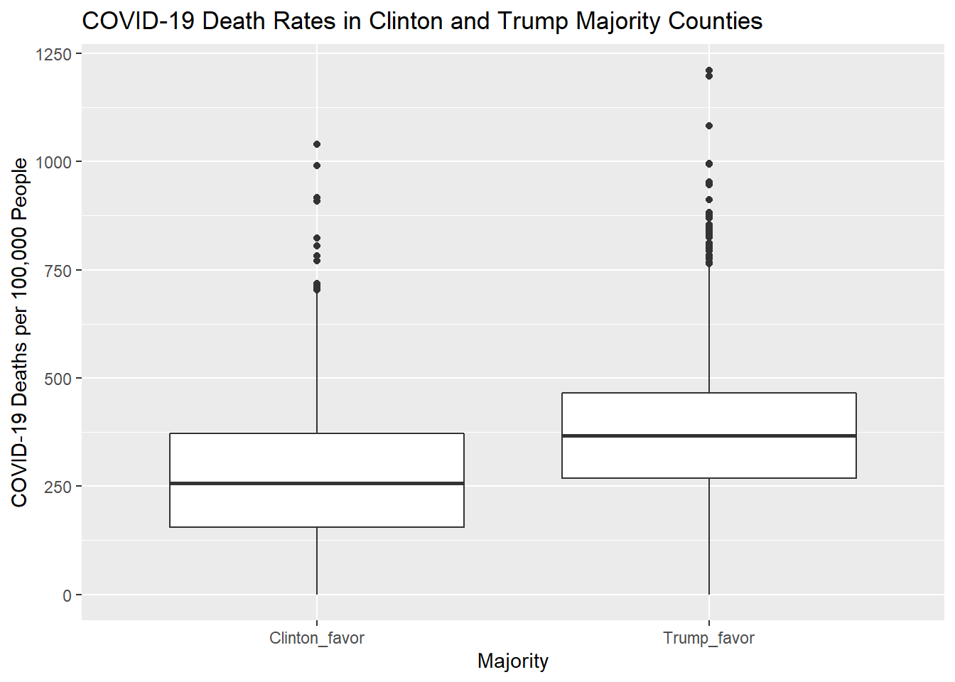
ggplot(na.omit(covid_vote_5), aes(x=majority, y=covid_death_rate))+geom_boxplot()+labs(x="Majority", y="COVID-19 Deaths per 100,000 People", title= "COVID-19 Death Rates in Clinton and Trump Majority Counties")

According to this boxplot, there appears to be a difference in median COVID-19 death rates based on if a county voted majority Trump of Clinton.

Modeling this Relationship

Below I try two different models including all of the control variables identified above. In the second model I omit counties where covid_death_rate is zero so I can log transform covid_death_rate. I think a log transformation could make sense in this case- perhaps only counties that had higher percentage Trump votes also had higher corresponding COVID-19 death rates (see scatterplot above).

#Model with covid_death_pct with 0 values included
summary(lm(covid_death_rate ~ percent_trump + over65_pct + med_income_2020 + Party+ Rural_urban_continuum_code_2013, data= covid_vote_5))


Call:
lm(formula = covid_death_rate ~ percent_trump + over65_pct + 
    med_income_2020 + Party + Rural_urban_continuum_code_2013, 
    data = covid_vote_5)

Residuals:
    Min      1Q  Median      3Q     Max 
-447.34  -82.23   -3.53   79.19  765.10 

Coefficients:
                                  Estimate Std. Error t value Pr(>|t|)    
(Intercept)                      5.406e+02  2.043e+01  26.463  < 2e-16 ***
percent_trump                    1.635e+02  1.778e+01   9.196  < 2e-16 ***
over65_pct                      -6.920e+01  5.964e+01  -1.160    0.246    
med_income_2020                 -4.955e-03  1.968e-04 -25.182  < 2e-16 ***
PartyRepublican                  2.536e+01  5.252e+00   4.829 1.44e-06 ***
Rural_urban_continuum_code_2013 -8.644e-01  1.160e+00  -0.745    0.456    
---
Signif. codes:  0 '***' 0.001 '**' 0.01 '*' 0.05 '.' 0.1 ' ' 1

Residual standard error: 138.6 on 3107 degrees of freedom
  (45 observations deleted due to missingness)
Multiple R-squared:  0.2668,    Adjusted R-squared:  0.2656 
F-statistic: 226.1 on 5 and 3107 DF,  p-value: < 2.2e-16

fit1<-lm(covid_death_rate ~ percent_trump + over65_pct + med_income_2020 + Party+ Rural_urban_continuum_code_2013, data= covid_vote_5)

#Model with covid_death_pct with 0 values excluded and logged covid_death_pct
summary(lm(log(covid_death_rate) ~ percent_trump + over65_pct + med_income_2020 + Party + Rural_urban_continuum_code_2013, data= covid_vote_5_no_zero))


Call:
lm(formula = log(covid_death_rate) ~ percent_trump + over65_pct + 
    med_income_2020 + Party + Rural_urban_continuum_code_2013, 
    data = covid_vote_5_no_zero)

Residuals:
     Min       1Q   Median       3Q      Max 
-3.15841 -0.19737  0.06346  0.27447  1.16727 

Coefficients:
                                  Estimate Std. Error t value Pr(>|t|)    
(Intercept)                      6.382e+00  6.656e-02  95.877  < 2e-16 ***
percent_trump                    7.718e-01  5.789e-02  13.331  < 2e-16 ***
over65_pct                      -2.974e-01  1.941e-01  -1.532  0.12557    
med_income_2020                 -1.720e-05  6.410e-07 -26.828  < 2e-16 ***
PartyRepublican                  5.297e-02  1.705e-02   3.106  0.00192 ** 
Rural_urban_continuum_code_2013 -1.826e-02  3.787e-03  -4.821  1.5e-06 ***
---
Signif. codes:  0 '***' 0.001 '**' 0.01 '*' 0.05 '.' 0.1 ' ' 1

Residual standard error: 0.4484 on 3085 degrees of freedom
  (1 observation deleted due to missingness)
Multiple R-squared:  0.2852,    Adjusted R-squared:  0.2841 
F-statistic: 246.2 on 5 and 3085 DF,  p-value: < 2.2e-16

fit2<-lm(log(covid_death_rate) ~ percent_trump + over65_pct + med_income_2020 + Party + Rural_urban_continuum_code_2013, data= covid_vote_5_no_zero)

The second model, where covid_death_rate is log transformed and the 66 observations where COVID-19 death rate is zero are omitted has the higher adjusted r-squared.

In both models, the coefficient of interest percent_trump, is significant at the 0.001 significance level and has a positive coefficient. This model suggests there is evidence that counties that vote higher for Trump experience higher COVID-19 death rates. Still, the adjusted R-squared is not very high.

Concerns with this model: - Potential multicollinearity between over65_pct and med_income_2020? and between gov dummy and percent trump? - why is the coefficient for percent over 65 negative?

Below I test a polynomial model (where at first death rate decreases and then decreases as the curved line in the scatterplot above), however, the adjusted R squared is still smaller than in the above model.

#polynomial model
summary(lm(covid_death_rate ~ poly(percent_trump, 2, raw=TRUE) + over65_pct + med_income_2020 + Party+ Rural_urban_continuum_code_2013, data= covid_vote_5))


Call:
lm(formula = covid_death_rate ~ poly(percent_trump, 2, raw = TRUE) + 
    over65_pct + med_income_2020 + Party + Rural_urban_continuum_code_2013, 
    data = covid_vote_5)

Residuals:
    Min      1Q  Median      3Q     Max 
-470.63  -82.97   -3.05   76.94  770.31 

Coefficients:
                                      Estimate Std. Error t value Pr(>|t|)    
(Intercept)                          6.393e+02  3.181e+01  20.093  < 2e-16 ***
poly(percent_trump, 2, raw = TRUE)1 -2.056e+02  9.310e+01  -2.209   0.0273 *  
poly(percent_trump, 2, raw = TRUE)2  3.286e+02  8.136e+01   4.039 5.50e-05 ***
over65_pct                          -4.899e+01  5.970e+01  -0.821   0.4120    
med_income_2020                     -5.004e-03  1.967e-04 -25.443  < 2e-16 ***
PartyRepublican                      2.273e+01  5.279e+00   4.305 1.72e-05 ***
Rural_urban_continuum_code_2013     -1.759e+00  1.178e+00  -1.492   0.1357    
---
Signif. codes:  0 '***' 0.001 '**' 0.01 '*' 0.05 '.' 0.1 ' ' 1

Residual standard error: 138.2 on 3106 degrees of freedom
  (45 observations deleted due to missingness)
Multiple R-squared:  0.2706,    Adjusted R-squared:  0.2692 
F-statistic:   192 on 6 and 3106 DF,  p-value: < 2.2e-16

fit3<-lm(covid_death_rate ~ poly(percent_trump, 2, raw=TRUE) + over65_pct + med_income_2020 + Party+ Rural_urban_continuum_code_2013, data= covid_vote_5)

Diagnositics

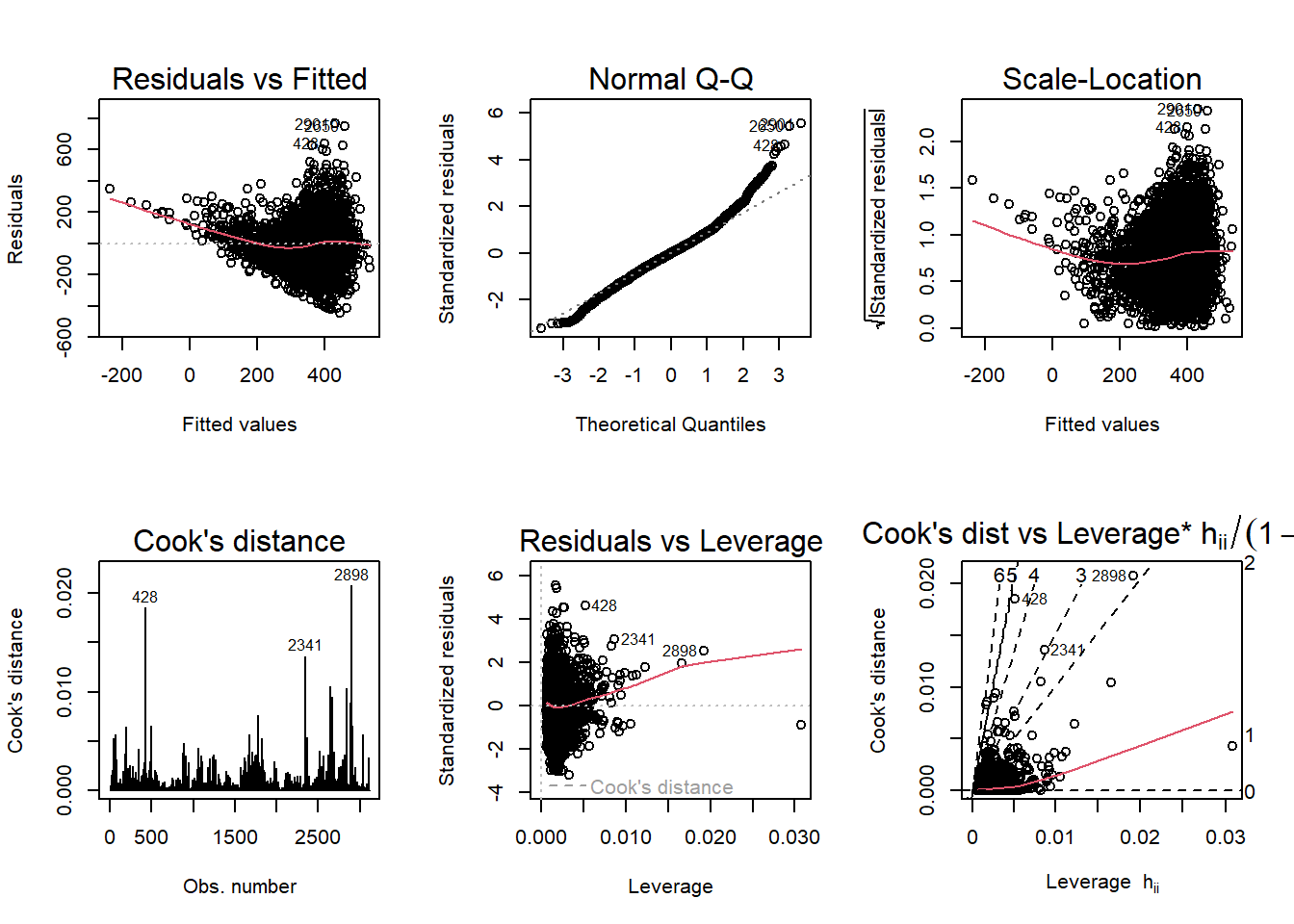
par(mfrow= c(2,3)); plot(fit1, which=1:6)

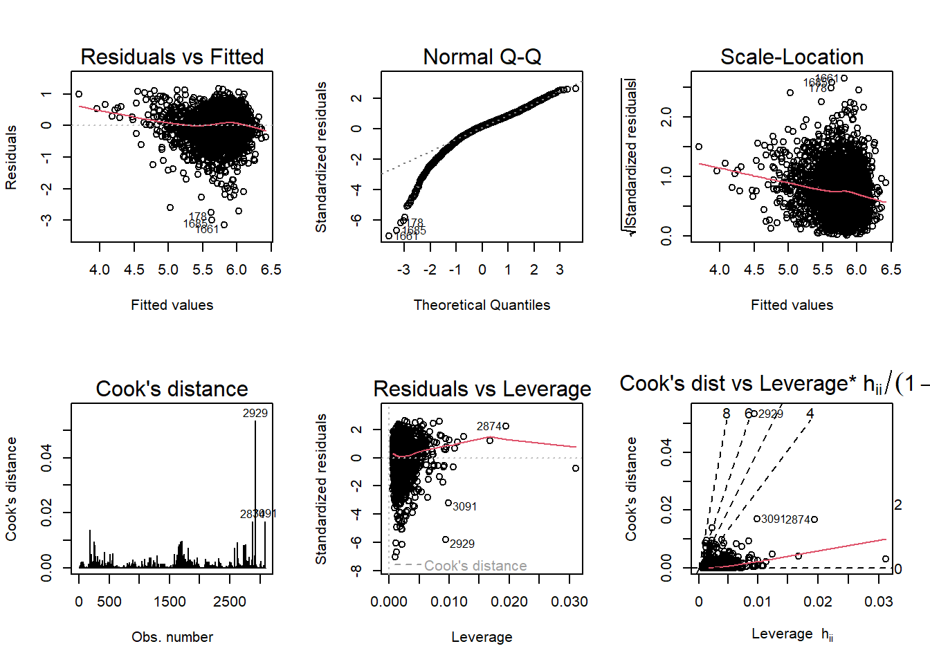
par(mfrow= c(2,3)); plot(fit2, which=1:6)

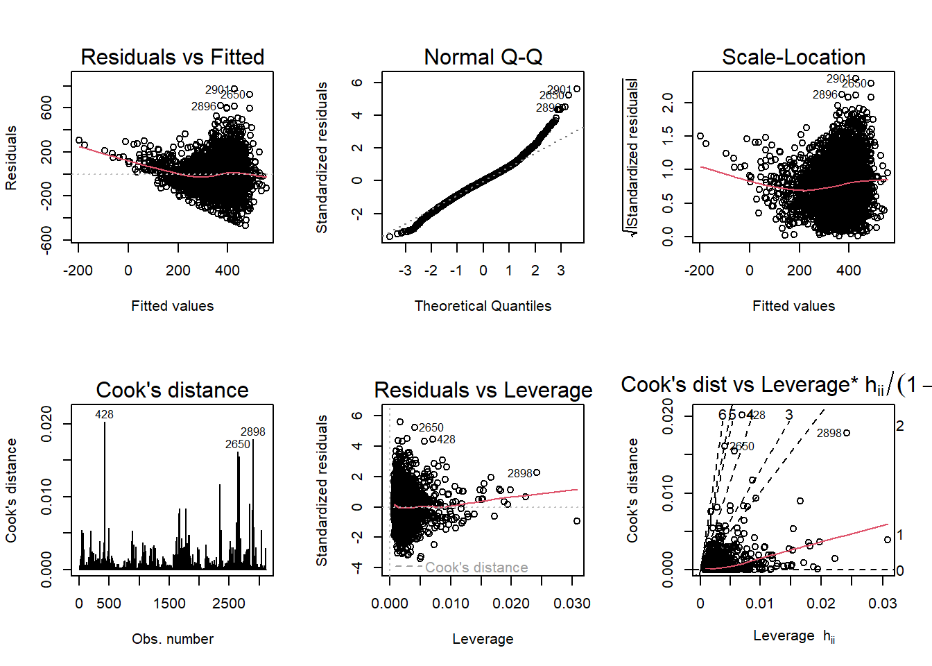
par(mfrow= c(2,3)); plot(fit3, which=1:6)

According to the diagnostic plots, none of the models seem to fit super well. For fit2, (the one where covid_death_rate is log transformed,) the residuals seem to have a trend (higher fitted values have lower residuals). Same with the Q-Q, plot, lower theoretical quantiles gave significantly lower standardized residuals. The scale location graph has a negative trend, suggesting variance may not be constant. There may be a couple outliers significantly affecting the model according 4/n which is approximately 0.0013. Residuals versus leverage looks ok, there does not appear to be any super concerning observations. Finally, Cooks dist to leverage 2898 has a high cooks distance and leverage and likely has a large influence on the model. The other models display similar issues.

Moving into part three of the project, I may look into other control variables that may improve the model or other transformations to improve R squared. Regardless there does not seem to be a super strong observable trend.

References

Ballotpedia. (2022). Partisan composition of governors. Accessed [November 10, 2022]. https://ballotpedia.org/Partisan_composition_of_governors

Economic Research Service. (2022). Unemployment and median household income for the U.S., States, and counties, 2000-2021. Accessed from the United States Department of Agriculture [November 10, 2022]. https://www.ers.usda.gov/data-products/county-level-data-sets/county-level-data-sets-download-data/

Jones, B. (2022). The Changing Political Geography of COVID-19 Over the Last Two Years. Pew Research Center. March 3, 2022. https://www.pewresearch.org/politics/2022/03/03/the-changing-political-geography-of-covid-19-over-the-last-two-years/

Mayo Clinic Staff. (2022). “COVID-19: Who’s at Higher Risk of Serious Symptoms?” Accessed from Mayo Clinic, [November 11, 2022]. https://www.mayoclinic.org/diseases-conditions/coronavirus/in-depth/coronavirus-who-is-at-risk/art-20483301

MIT Election Data and Science Lab. (2021) County Presidential Election Returns 2000-2020. Accessed from the Harvard Dataverse [October 11, 2022]. https://doi.org/10.7910/DVN/VOQCHQ

National Center for Health Statistics. (2022). Provisional COVID-19 Deaths by County, and Race and Hispanic Origin. Accessed from the Centers for Disease Control [October 11, 2022]. https://data.cdc.gov/d/k8wy-p9cg

USA Facts. (2022).US COVID-19 cases and deaths by state. Accessed [November 10, 2022]. https://usafacts.org/visualizations/coronavirus-covid-19-spread-map/?utm_source=usnews&utm_medium=partnership&utm_campaign=2020&utm_content=healthiestcommunitiescovid

United States Census Bureau. (2019). Annual County Resident Population Estimates by Age, Sex, Race, and Hispanic Origin: April 1, 2010 to July 1, 2019 (CC-EST2019-ALLDATA). Accessed from Census.gov [November 11, 2022].https://www.census.gov/data/tables/time-series/demo/popest/2010s-counties-detail.html

Wood, D. and Brumfiel, G. (2021). Pro-Trump counties now have far higher COVID death rates. Misinformation is to blame. NPR. December 5, 2021. https://www.npr.org/sections/health-shots/2021/12/05/1059828993/data-vaccine-misinformation-trump-counties-covid-death-rate

[Need to add italics to references]