Code
library(tidyverse)
library(ggplot2)
library(stats)
library(reshape2)
library(skimr)
library(randomForest)
library(caret)
library(interactions)
library(lmtest)
library(sandwich)
library(plotly)

knitr::opts_chunk$set(echo = TRUE)Mani Shanker Kamarapu
November 11, 2022
Churning refers to a customer who leaves one company to go to another company. Customer churn introduces not only some loss in income but also other negative effects on the operation of companies. Churn management is the concept of identifying those customers who are intending to move their custom to a competing service provider.
Risselada et al. (2010) stated that churn management is becoming part of customer relationship management. It is important for companies to consider it as they try to establish long-term relationships with customers and maximize the value of their customer base.
A. Does churn-rate depend on the geographical factors(Customer’s location) of the customer?
B. Do non-active members are probable to churn or not?
This project will be useful to better understand more about the customer difficulties and factors and also give us a pretty good idea on the factors effecting the customers to exit and also about the dormant state of the customers.
Customer churn analysis has become a major concern in almost every industry that offers products and services. The model developed will help banks identify clients who are likely to be churners and develop appropriate marketing actions to retain their valuable clients. And this model also supports information about similar customer group to consider which marketing reactions are to be provided. Thus, due to existing customers are retained, it will provide banks with increased profits and revenues. By the end of this article, let’s attempt to solve some of the key business challenges pertaining to customer attrition like say, (1) what is the likelihood of an active customer leaving an organization? (2) what are key indicators of a customer churn? (3) what retention strategies can be implemented based on the results to diminish prospective customer churn?
Given the above, we can frame our hypotheses as follows:
Customer’s location will not be statistically predict the churn-rate.
Customer’s location will be statistically predict the churn-rate.
I believe that the customer’s location have an effect on customer’s churn rate as based on location there is statistical difference in customer’s salary and balance.
Active members will not churn.
Active members will churn.
I think that inactive members are more likely to exit rather than active members as there is a high chance of them churning out as they are are inactive for a longtime.
Rows: 10000 Columns: 14
── Column specification ────────────────────────────────────────────────────────
Delimiter: ","
chr  (3): Surname, Geography, Gender
dbl (11): RowNumber, CustomerId, CreditScore, Age, Tenure, Balance, NumOfPro...

ℹ Use `spec()` to retrieve the full column specification for this data.
ℹ Specify the column types or set `show_col_types = FALSE` to quiet this message.This data set is originated from a U.S. bank and is downloaded from kaggle. This data set includes 10k bank customer data records with 14 attributes including socio-demographic attributes, account level and behavioral attributes.
The response variable is Exited variable and the main explanatory variables are Geography and IsActiveMember. And the other explanatory variables are Credit Score, Gender, Age and Balance.
spc_tbl_ [10,000 × 14] (S3: spec_tbl_df/tbl_df/tbl/data.frame)
 $ RowNumber      : num [1:10000] 1 2 3 4 5 6 7 8 9 10 ...
 $ CustomerId     : num [1:10000] 15634602 15647311 15619304 15701354 15737888 ...
 $ Surname        : chr [1:10000] "Hargrave" "Hill" "Onio" "Boni" ...
 $ CreditScore    : num [1:10000] 619 608 502 699 850 645 822 376 501 684 ...
 $ Geography      : chr [1:10000] "France" "Spain" "France" "France" ...
 $ Gender         : chr [1:10000] "Female" "Female" "Female" "Female" ...
 $ Age            : num [1:10000] 42 41 42 39 43 44 50 29 44 27 ...
 $ Tenure         : num [1:10000] 2 1 8 1 2 8 7 4 4 2 ...
 $ Balance        : num [1:10000] 0 83808 159661 0 125511 ...
 $ NumOfProducts  : num [1:10000] 1 1 3 2 1 2 2 4 2 1 ...
 $ HasCrCard      : num [1:10000] 1 0 1 0 1 1 1 1 0 1 ...
 $ IsActiveMember : num [1:10000] 1 1 0 0 1 0 1 0 1 1 ...
 $ EstimatedSalary: num [1:10000] 101349 112543 113932 93827 79084 ...
 $ Exited         : num [1:10000] 1 0 1 0 0 1 0 1 0 0 ...
 - attr(*, "spec")=
  .. cols(
  ..   RowNumber = col_double(),
  ..   CustomerId = col_double(),
  ..   Surname = col_character(),
  ..   CreditScore = col_double(),
  ..   Geography = col_character(),
  ..   Gender = col_character(),
  ..   Age = col_double(),
  ..   Tenure = col_double(),
  ..   Balance = col_double(),
  ..   NumOfProducts = col_double(),
  ..   HasCrCard = col_double(),
  ..   IsActiveMember = col_double(),
  ..   EstimatedSalary = col_double(),
  ..   Exited = col_double()
  .. )
- attr(*, "problems")=<externalptr> RowNumber CustomerId Surname CreditScore
Min. : 1 Min. :15565701 Length:10000 Min. :350.0
1st Qu.: 2501 1st Qu.:15628528 Class :character 1st Qu.:584.0
Median : 5000 Median :15690738 Mode :character Median :652.0
Mean : 5000 Mean :15690941 Mean :650.5
3rd Qu.: 7500 3rd Qu.:15753234 3rd Qu.:718.0
Max. :10000 Max. :15815690 Max. :850.0
Geography Gender Age Tenure
Length:10000 Length:10000 Min. :18.00 Min. : 0.000
Class :character Class :character 1st Qu.:32.00 1st Qu.: 3.000
Mode :character Mode :character Median :37.00 Median : 5.000
Mean :38.92 Mean : 5.013
3rd Qu.:44.00 3rd Qu.: 7.000
Max. :92.00 Max. :10.000
Balance NumOfProducts HasCrCard IsActiveMember
Min. : 0 Min. :1.00 Min. :0.0000 Min. :0.0000
1st Qu.: 0 1st Qu.:1.00 1st Qu.:0.0000 1st Qu.:0.0000
Median : 97199 Median :1.00 Median :1.0000 Median :1.0000
Mean : 76486 Mean :1.53 Mean :0.7055 Mean :0.5151
3rd Qu.:127644 3rd Qu.:2.00 3rd Qu.:1.0000 3rd Qu.:1.0000
Max. :250898 Max. :4.00 Max. :1.0000 Max. :1.0000
EstimatedSalary Exited
Min. : 11.58 Min. :0.0000
1st Qu.: 51002.11 1st Qu.:0.0000
Median :100193.91 Median :0.0000
Mean :100090.24 Mean :0.2037
3rd Qu.:149388.25 3rd Qu.:0.0000
Max. :199992.48 Max. :1.0000 Rows: 10,000
Columns: 14
$ RowNumber <dbl> 1, 2, 3, 4, 5, 6, 7, 8, 9, 10, 11, 12, 13, 14, 15, 16,…
$ CustomerId <dbl> 15634602, 15647311, 15619304, 15701354, 15737888, 1557…
$ Surname <chr> "Hargrave", "Hill", "Onio", "Boni", "Mitchell", "Chu",…
$ CreditScore <dbl> 619, 608, 502, 699, 850, 645, 822, 376, 501, 684, 528,…
$ Geography <chr> "France", "Spain", "France", "France", "Spain", "Spain…
$ Gender <chr> "Female", "Female", "Female", "Female", "Female", "Mal…
$ Age <dbl> 42, 41, 42, 39, 43, 44, 50, 29, 44, 27, 31, 24, 34, 25…
$ Tenure <dbl> 2, 1, 8, 1, 2, 8, 7, 4, 4, 2, 6, 3, 10, 5, 7, 3, 1, 9,…
$ Balance <dbl> 0.00, 83807.86, 159660.80, 0.00, 125510.82, 113755.78,…
$ NumOfProducts <dbl> 1, 1, 3, 2, 1, 2, 2, 4, 2, 1, 2, 2, 2, 2, 2, 2, 1, 2, …
$ HasCrCard <dbl> 1, 0, 1, 0, 1, 1, 1, 1, 0, 1, 0, 1, 1, 0, 1, 0, 1, 1, …
$ IsActiveMember <dbl> 1, 1, 0, 0, 1, 0, 1, 0, 1, 1, 0, 0, 0, 0, 1, 1, 0, 1, …
$ EstimatedSalary <dbl> 101348.88, 112542.58, 113931.57, 93826.63, 79084.10, 1…
$ Exited <dbl> 1, 0, 1, 0, 0, 1, 0, 1, 0, 0, 0, 0, 0, 0, 0, 0, 1, 0, …Dimensions of the data set
The data set has 10000 rows and 11 columns now after removing the first 3 columns which are not necessary for analysis and will not effect the model.
Checking for Null values
From above box plot, Credit score variable has few outliers, but they cannot potentially affect the data set.
From above box plot, age variable has outliers (age group above 60 constitutes outliers), however there are few outliers. But they cannot potentially affect the data set.
From above box plot, Tenure variable has no outliers.
From above box plot, Balance variable has no outliers.
From above box plot, NumofProducts variable has no outliers.
From above box plot, EstimatedSalary variable has no outliers.
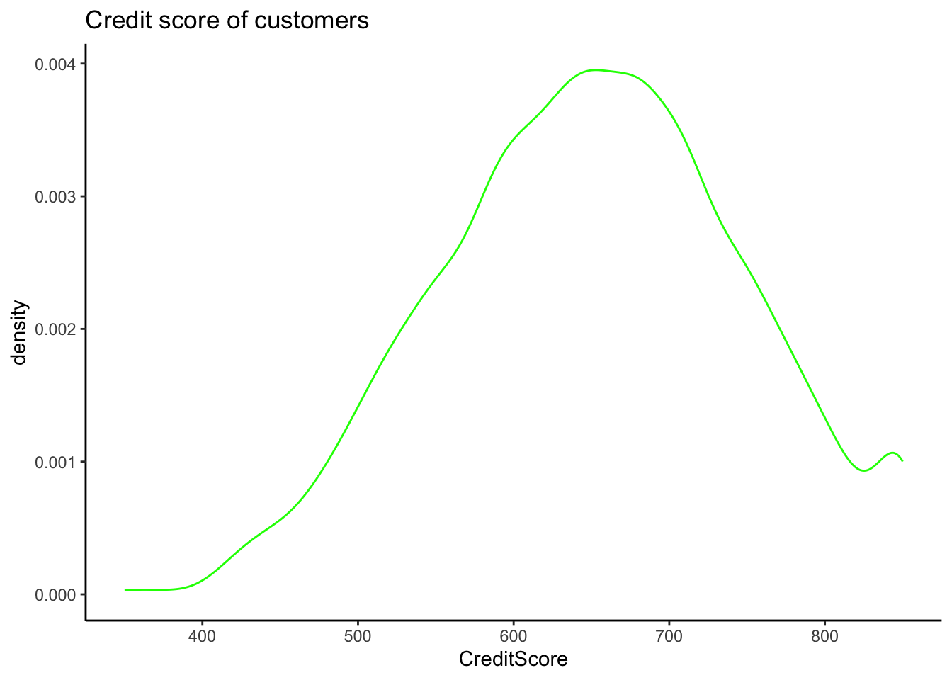
The credit score is looking to be normal with median in range of 650-700.
Churn %>%
group_by(Geography) %>% # Variable to be transformed
count() %>%
ungroup() %>%
mutate(perc = `n` / sum(`n`)) %>%
arrange(perc) %>%
mutate(labels = scales::percent(perc)) %>%
ggplot(aes(x = "", y = perc, fill = Geography)) +
ggtitle("Location of customers") +
geom_col(color = "black") +
geom_label(aes(label = labels), color = c(1, "white", "white"),
position = position_stack(vjust = 0.5),
show.legend = FALSE) +
guides(fill = guide_legend(title = "Geography")) +
scale_fill_viridis_d() +
coord_polar(theta = "y") +
theme_void()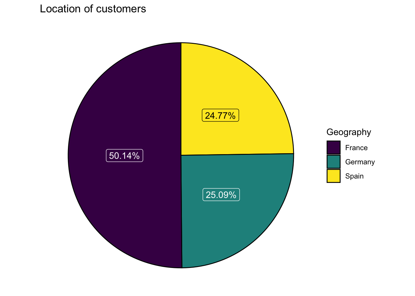
<ggproto object: Class ScaleDiscrete, Scale, gg>
aesthetics: fill
axis_order: function
break_info: function
break_positions: function
breaks: waiver
call: call
clone: function
dimension: function
drop: TRUE
expand: waiver
get_breaks: function
get_breaks_minor: function
get_labels: function
get_limits: function
guide: legend
is_discrete: function
is_empty: function
labels: waiver
limits: NULL
make_sec_title: function
make_title: function
map: function
map_df: function
n.breaks.cache: NULL
na.translate: TRUE
na.value: NA
name: waiver
palette: function
palette.cache: NULL
position: left
range: <ggproto object: Class RangeDiscrete, Range, gg>
range: NULL
reset: function
train: function
super: <ggproto object: Class RangeDiscrete, Range, gg>
rescale: function
reset: function
scale_name: brewer
train: function
train_df: function
transform: function
transform_df: function
super: <ggproto object: Class ScaleDiscrete, Scale, gg>The Geography variable consists of 3 values, i.e, France(50%), Germany(25%) and Spain(25%).
The Gender variable consists of Male and Female values and male count(5457) is more than female count(4543).
The tenure of all customers is between 0-10 years and is almost equal no of customers in each year.
`stat_bin()` using `bins = 30`. Pick better value with `binwidth`.We have a lot of people with balance as zero but if we ignore that the other values form a normal at 120000 in median.
Churn %>%
group_by(NumOfProducts) %>% # Variable to be transformed
count() %>%
ungroup() %>%
mutate(perc = `n` / sum(`n`)) %>%
arrange(perc) %>%
mutate(labels = scales::percent(perc)) %>%
ggplot(aes(x = "", y = perc, fill = as.factor(NumOfProducts))) +
ggtitle("No of products owned by customers") +
geom_col(color = "black") +
geom_label(aes(label = labels), color = c(1, "white", "white", "white"),
position = position_stack(vjust = 0.5),
show.legend = FALSE) +
guides(fill = guide_legend(title = "NumofProducts")) +
scale_fill_viridis_d() +
coord_polar(theta = "y") +
theme_void()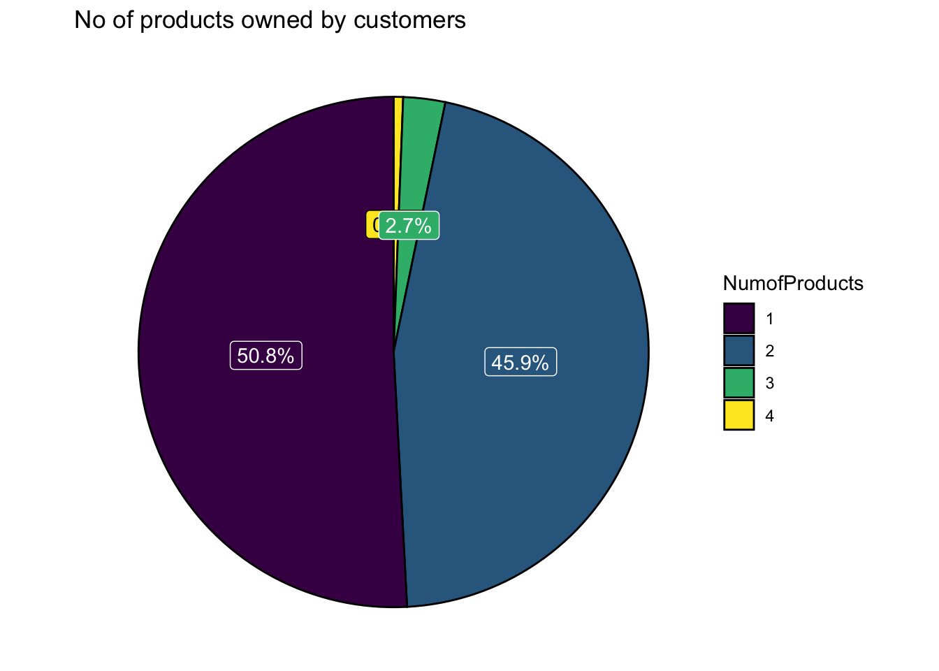
<ggproto object: Class ScaleDiscrete, Scale, gg>
aesthetics: fill
axis_order: function
break_info: function
break_positions: function
breaks: waiver
call: call
clone: function
dimension: function
drop: TRUE
expand: waiver
get_breaks: function
get_breaks_minor: function
get_labels: function
get_limits: function
guide: legend
is_discrete: function
is_empty: function
labels: waiver
limits: NULL
make_sec_title: function
make_title: function
map: function
map_df: function
n.breaks.cache: NULL
na.translate: TRUE
na.value: NA
name: waiver
palette: function
palette.cache: NULL
position: left
range: <ggproto object: Class RangeDiscrete, Range, gg>
range: NULL
reset: function
train: function
super: <ggproto object: Class RangeDiscrete, Range, gg>
rescale: function
reset: function
scale_name: brewer
train: function
train_df: function
transform: function
transform_df: function
super: <ggproto object: Class ScaleDiscrete, Scale, gg>According to above plot, the maximum no of the products owned by customers is 4 and minimum is 1. Majority of customers own either 1 or 2 products.
According to above plot, 7055 customers have credit card and 2945 customers does not have credit card.
Form the above plot, it looks like there are as many inactive members(4849) as active members(5151).
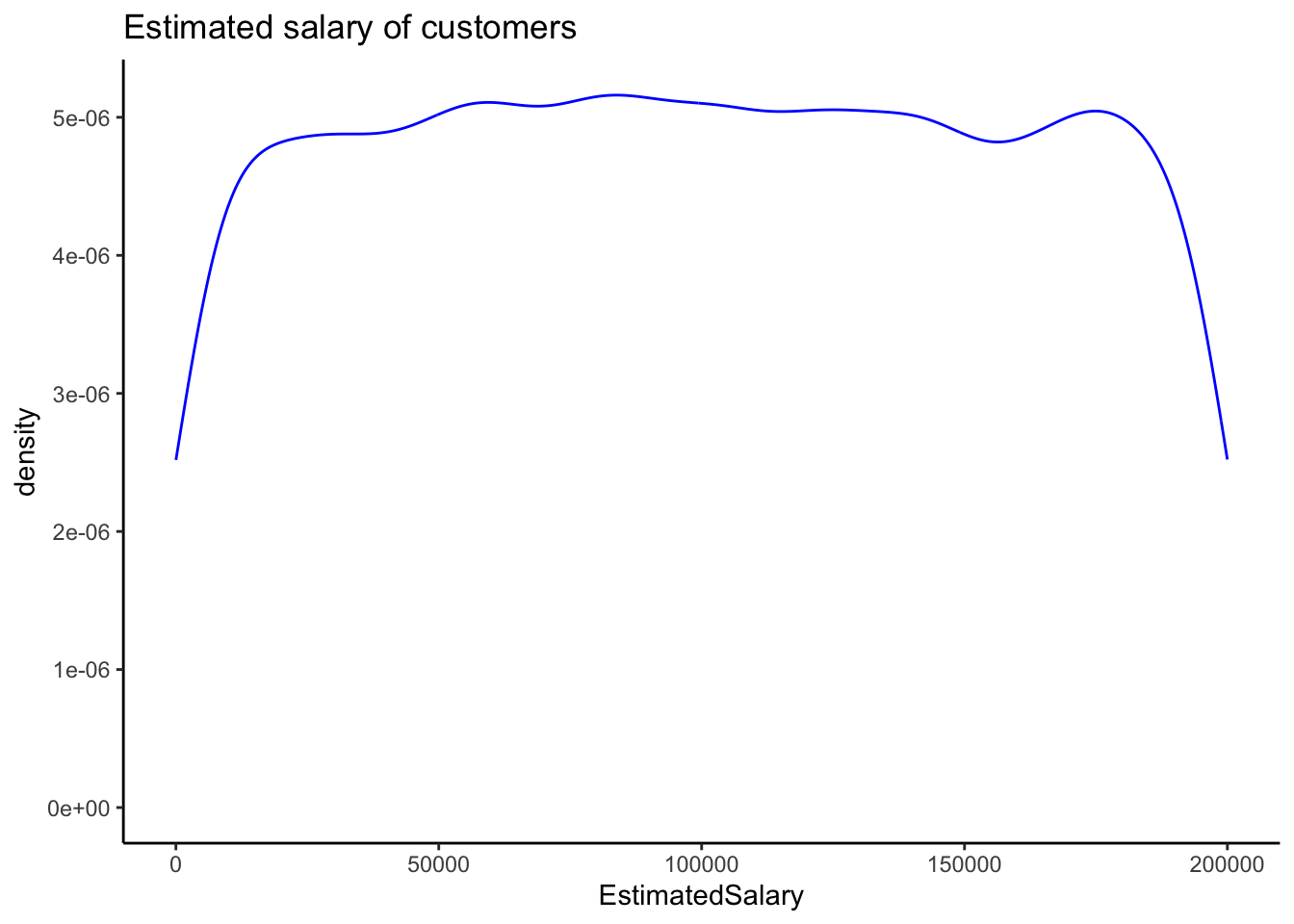
From above graph, the data set contains the customers of all types of income from 0-200000.
Churn %>%
group_by(Exited) %>% # Variable to be transformed
count() %>%
ungroup() %>%
mutate(perc = `n` / sum(`n`)) %>%
arrange(perc) %>%
mutate(labels = scales::percent(perc)) %>%
ggplot(aes(x = "", y = perc, fill = as.factor(Exited))) +
ggtitle("Churn-rate of customers") +
geom_col(color = "black") +
geom_label(aes(label = labels), color = c(1, "white"),
position = position_stack(vjust = 0.5),
show.legend = FALSE) +
guides(fill = guide_legend(title = "Churn-rate")) +
scale_fill_viridis_d() +
coord_polar(theta = "y") +
theme_void()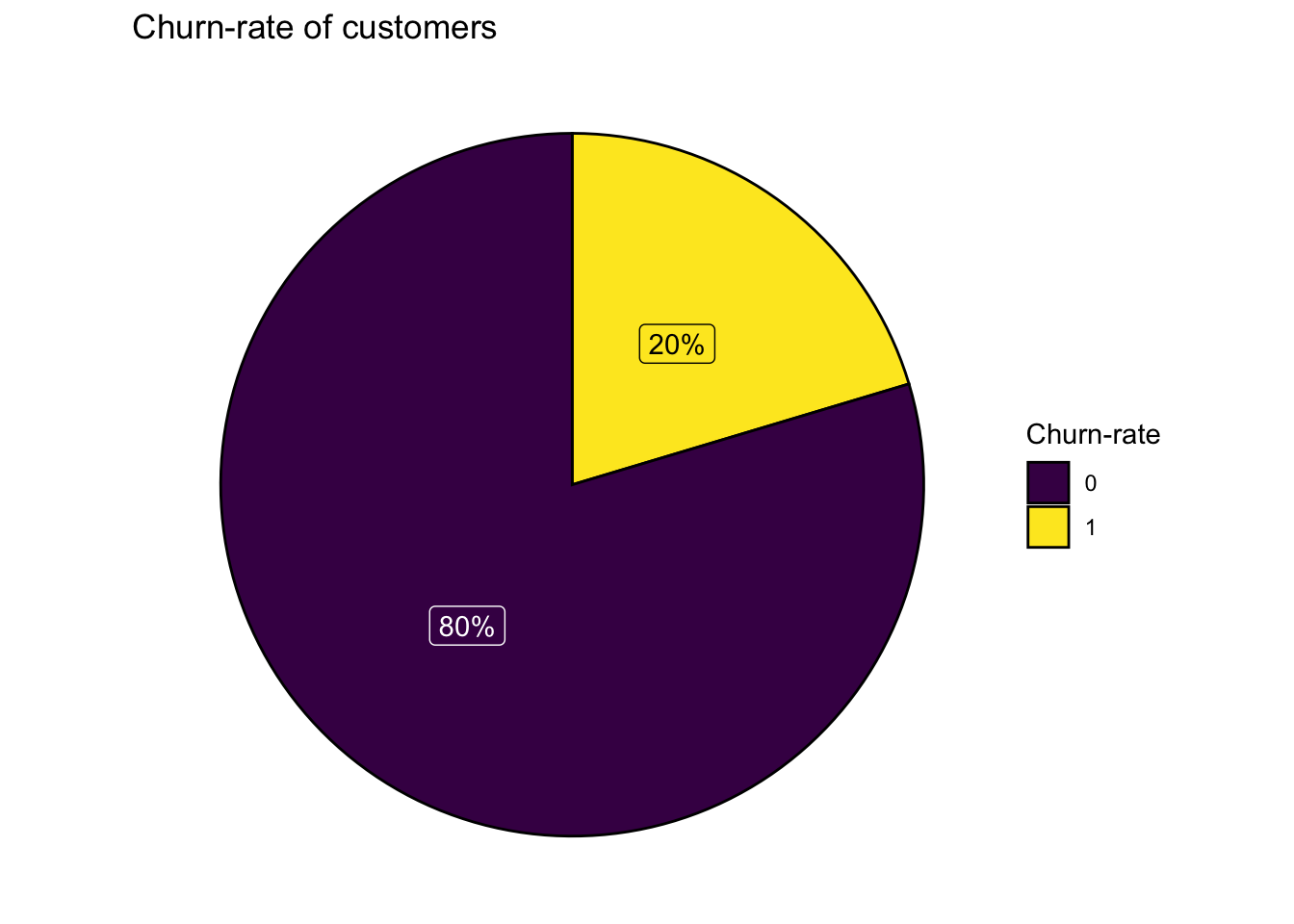
<ggproto object: Class ScaleDiscrete, Scale, gg>
aesthetics: fill
axis_order: function
break_info: function
break_positions: function
breaks: waiver
call: call
clone: function
dimension: function
drop: TRUE
expand: waiver
get_breaks: function
get_breaks_minor: function
get_labels: function
get_limits: function
guide: legend
is_discrete: function
is_empty: function
labels: waiver
limits: NULL
make_sec_title: function
make_title: function
map: function
map_df: function
n.breaks.cache: NULL
na.translate: TRUE
na.value: NA
name: waiver
palette: function
palette.cache: NULL
position: left
range: <ggproto object: Class RangeDiscrete, Range, gg>
range: NULL
reset: function
train: function
super: <ggproto object: Class RangeDiscrete, Range, gg>
rescale: function
reset: function
scale_name: brewer
train: function
train_df: function
transform: function
transform_df: function
super: <ggproto object: Class ScaleDiscrete, Scale, gg>From the pie chart, 80% of customers are not churned and 20% have already exited.
temp <- Churn %>%
select(-c(Geography, Gender))
round(cor(temp),3) %>%
melt() %>%
ggplot(aes(x=Var1, y=Var2, fill=value)) +
geom_tile() +
geom_text(aes(Var2, Var1, label = value), color = "black", size = 4) +
labs(x = NULL, y = NULL) +
ggtitle("Correlation plot") +
theme(axis.text.x = element_text(angle = 90))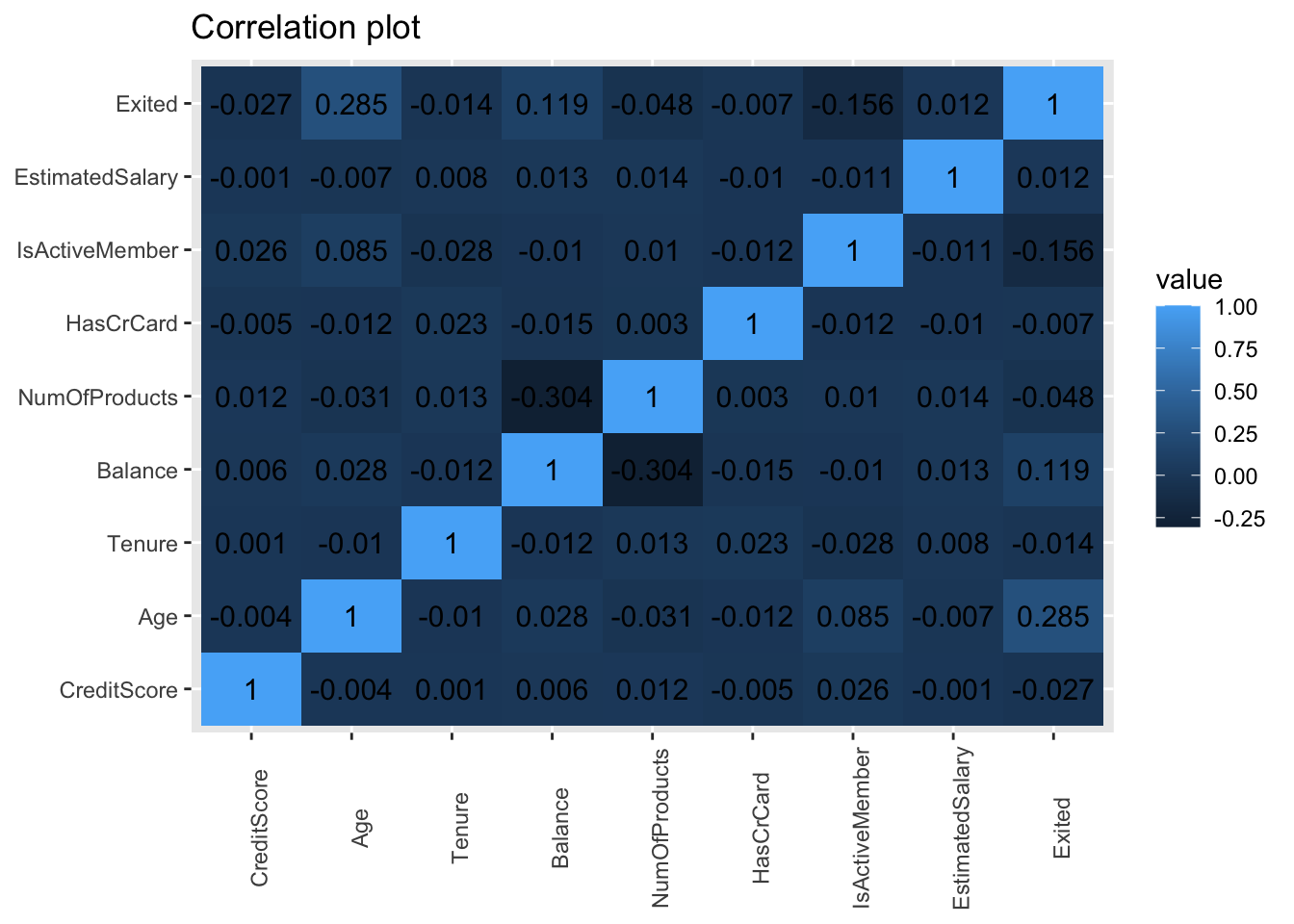
Churn has a positive correlation with age, balance and estimated salary. Generally the correlation coefficients are not so high.
There are 4 categorical variables in the data set as follows:
Majority of the data is from persons from France. However, the proportion of churned customers is with inversely related to the population of customers alluding to the bank possibly having a problem (maybe not enough customer service resources allocated) in the areas where it has fewer clients.
The proportion of female customers churning is also greater than that of male customers.
Majority of the customers that churned are those with credit cards. Given that majority of the customers have credit cards could prove this to be just a coincidence.
Unsurprisingly the inactive members have a greater churn. Worryingly is that the overall proportion of inactive mebers is quite high suggesting that the bank may need a program implemented to turn this group to active customers as this will definately have a positive impact on the customer churn.
There are 6 continuous variables in the data set as follows:
There is no significant difference in the credit score distribution between retained and churned customers.
The older customers are churning at more rate than the younger ones alluding to a difference in service preference in the age categories. The bank may need to review their target market or review the strategy for retention between the different age groups.
With regard to the tenure, the clients on either extreme end (spent little time with the bank or a lot of time with the bank) are more likely to churn compared to those that are of average tenure.
The bank is losing customers with significant bank balances which is likely to hit their available capital for lending.
The no of products not has a significant effect on the likelihood to churn.
The Estimated salary not has a significant effect on the likelihood to churn.
Call:
lm(formula = Exited ~ as.factor(IsActiveMember), data = Churn)
Residuals:
Min 1Q Median 3Q Max
-0.2685 -0.2685 -0.1427 -0.1427 0.8573
Coefficients:
Estimate Std. Error t value Pr(>|t|)
(Intercept) 0.268509 0.005713 47.0 <2e-16 ***
as.factor(IsActiveMember)1 -0.125818 0.007961 -15.8 <2e-16 ***
---
Signif. codes: 0 '***' 0.001 '**' 0.01 '*' 0.05 '.' 0.1 ' ' 1
Residual standard error: 0.3978 on 9998 degrees of freedom
Multiple R-squared: 0.02438, Adjusted R-squared: 0.02428
F-statistic: 249.8 on 1 and 9998 DF, p-value: < 2.2e-16
Call:
lm(formula = Exited ~ ., data = Churn)
Residuals:
Min 1Q Median 3Q Max
-0.84083 -0.23374 -0.12020 0.03515 1.20544
Coefficients:
Estimate Std. Error t value Pr(>|t|)
(Intercept) -8.034e-02 3.372e-02 -2.382 0.0172 *
CreditScore -9.386e-05 3.844e-05 -2.441 0.0146 *
GeographyGermany 1.262e-01 9.915e-03 12.728 < 2e-16 ***
GeographySpain 4.043e-03 9.123e-03 0.443 0.6577
GenderMale -7.455e-02 7.470e-03 -9.980 < 2e-16 ***
Age 1.110e-02 3.562e-04 31.165 < 2e-16 ***
Tenure -1.906e-03 1.285e-03 -1.483 0.1381
Balance 3.139e-07 6.881e-08 4.562 5.12e-06 ***
NumOfProducts -1.577e-02 6.764e-03 -2.331 0.0198 *
HasCrCard -4.944e-03 8.154e-03 -0.606 0.5443
IsActiveMember -1.411e-01 7.470e-03 -18.891 < 2e-16 ***
EstimatedSalary 6.850e-08 6.461e-08 1.060 0.2890
---
Signif. codes: 0 '***' 0.001 '**' 0.01 '*' 0.05 '.' 0.1 ' ' 1
Residual standard error: 0.3714 on 9988 degrees of freedom
Multiple R-squared: 0.1508, Adjusted R-squared: 0.1499
F-statistic: 161.2 on 11 and 9988 DF, p-value: < 2.2e-16
Call:
lm(formula = Exited ~ Geography, data = Churn)
Residuals:
Min 1Q Median 3Q Max
-0.3244 -0.1667 -0.1615 -0.1615 0.8385
Coefficients:
Estimate Std. Error t value Pr(>|t|)
(Intercept) 0.161548 0.005602 28.836 <2e-16 ***
GeographyGermany 0.162884 0.009701 16.791 <2e-16 ***
GeographySpain 0.005186 0.009743 0.532 0.595
---
Signif. codes: 0 '***' 0.001 '**' 0.01 '*' 0.05 '.' 0.1 ' ' 1
Residual standard error: 0.3967 on 9997 degrees of freedom
Multiple R-squared: 0.03013, Adjusted R-squared: 0.02993
F-statistic: 155.3 on 2 and 9997 DF, p-value: < 2.2e-16Summarizing the above three models, the model1 describes the regression between Exited and Active member and secone model predicts the churn rate based on all the variables and third model is analysis between exited and geography. And model1 and model3 seems to be significant proving our hypothesis.
Call:
lm(formula = Exited ~ . - Geography - HasCrCard - NumOfProducts -
EstimatedSalary - Tenure, data = Churn)
Residuals:
Min 1Q Median 3Q Max
-0.7805 -0.2361 -0.1251 0.0271 1.1939
Coefficients:
Estimate Std. Error t value Pr(>|t|)
(Intercept) -1.144e-01 2.977e-02 -3.843 0.000122 ***
CreditScore -9.307e-05 3.877e-05 -2.401 0.016388 *
GenderMale -7.748e-02 7.529e-03 -10.291 < 2e-16 ***
Age 1.132e-02 3.588e-04 31.539 < 2e-16 ***
Balance 7.081e-07 6.007e-08 11.789 < 2e-16 ***
IsActiveMember -1.430e-01 7.528e-03 -18.999 < 2e-16 ***
---
Signif. codes: 0 '***' 0.001 '**' 0.01 '*' 0.05 '.' 0.1 ' ' 1
Residual standard error: 0.3746 on 9994 degrees of freedom
Multiple R-squared: 0.1356, Adjusted R-squared: 0.1352
F-statistic: 313.5 on 5 and 9994 DF, p-value: < 2.2e-16In the model4, I have used backward elimination process by removing the highest p values to get a significant model and it is significant after removing above 5 variables removed in call.
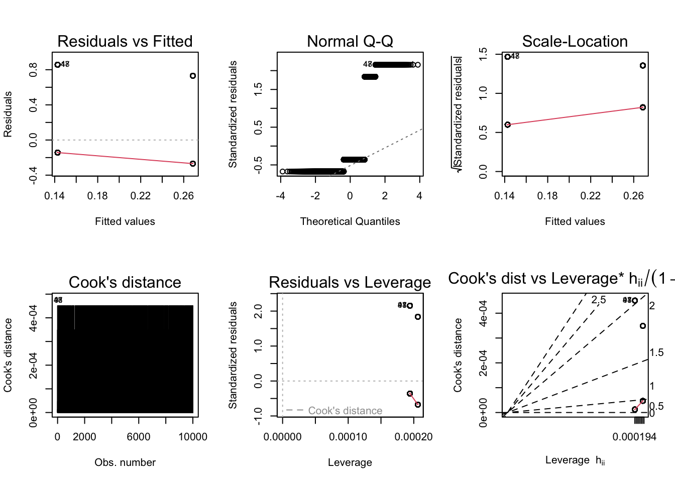
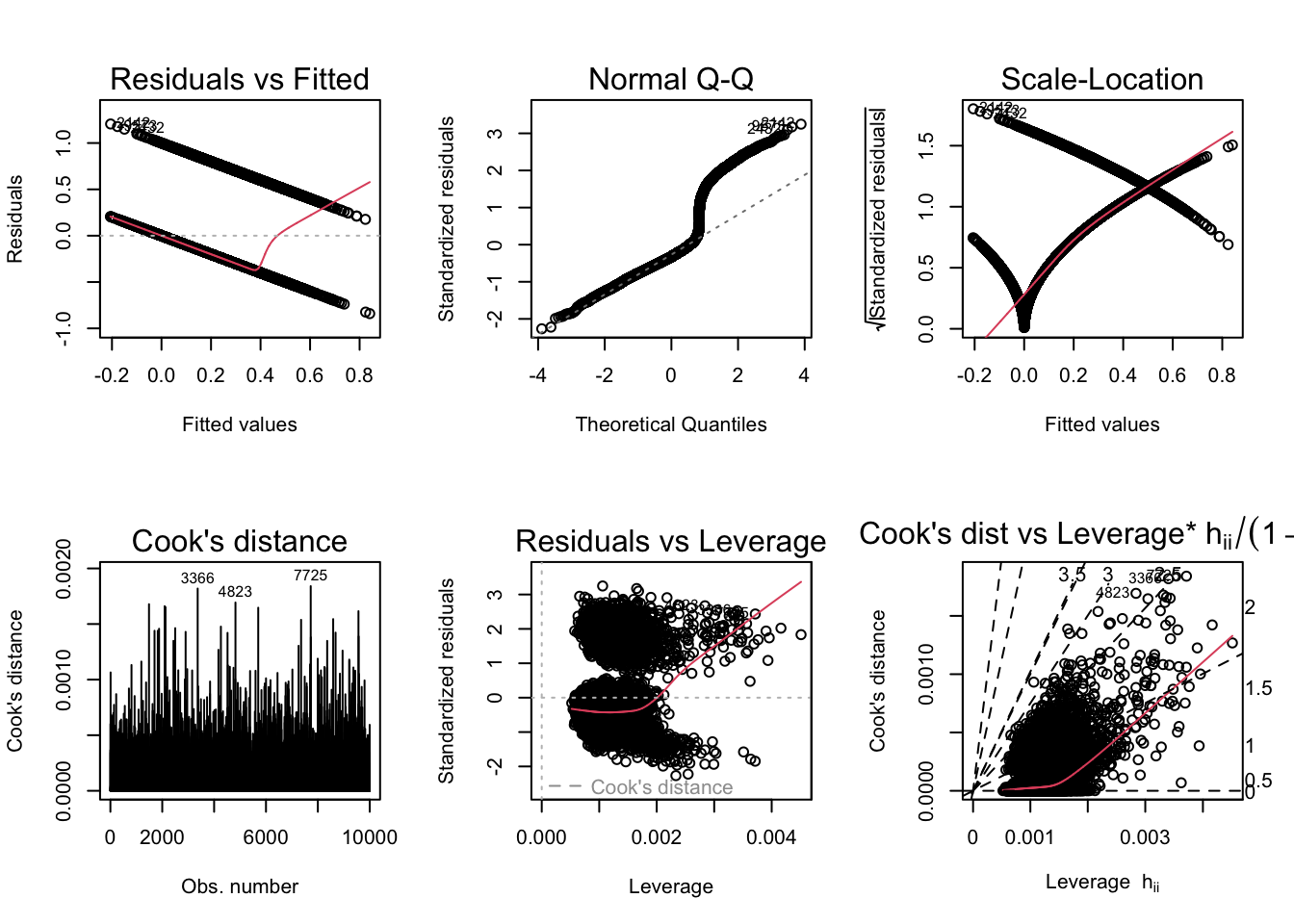
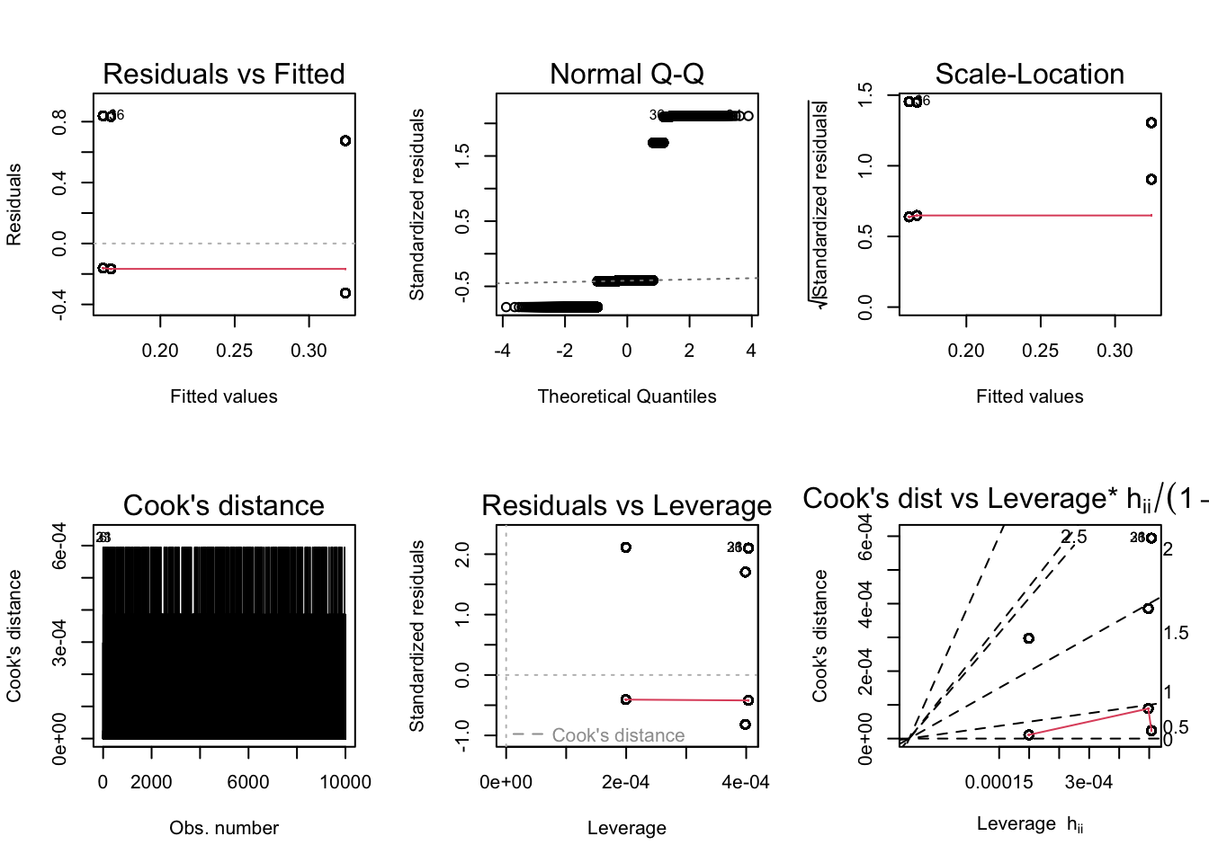
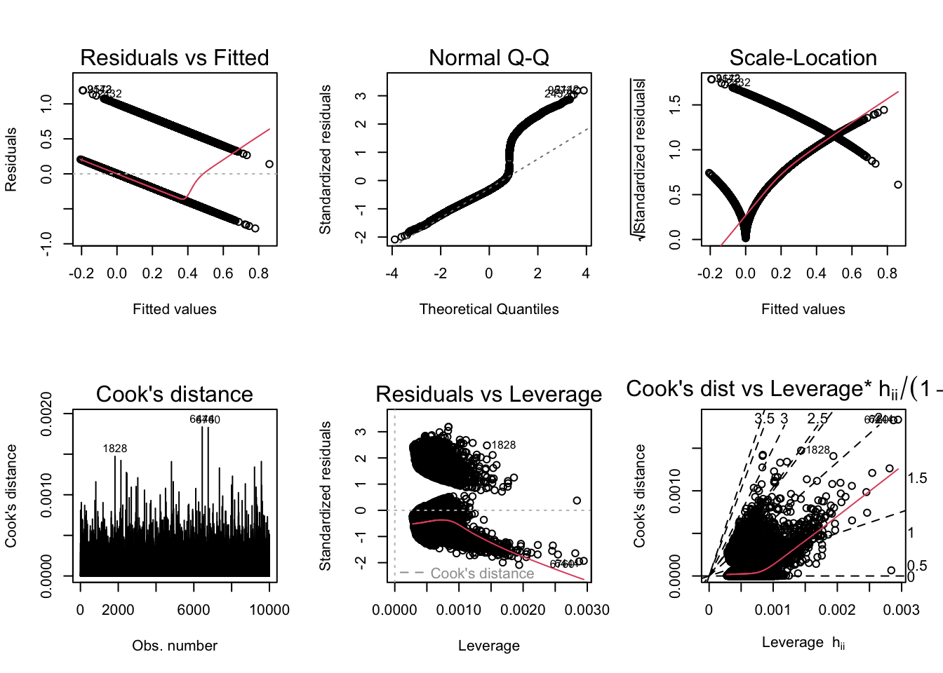
According to the diagnostic plots, none of the models seem to fit super well. There are violations of assumptions in models. In some the residuals seem to have a trend (higher fitted values have lower residuals). Same with the Q-Q, plot, lower theoretical quantiles gave significantly lower standardized residuals. The scale location graph has a negative trend, suggesting variance may not be constant. Cooks dist to leverage has a high cooks distance and leverage and likely has a large influence on the model. The other models display similar issues.
Moving into part three of the project, I may look into other control variables that may improve the model or other transformations to improve R squared. I would try the logistic regression and randomforest models and check them in part3.
Chicco, D. & Jurman, G., 2020. The advantages of the Matthews correlation coefficient (MCC) over F1 score and accuracy in binary classification evaluation. BMC genomics, 21(1), pp. 6-13.
Colgate, M., Stewart, K. & Kinsella, R., 1996. Customer Defection: A study of the student market in Ireland. International Journal of Bank Marketing, 14(3), pp. 23-29.
De Caigny, A., Coussement, K. & De Bock, K. W., 2018. A new hybrid classification algorithm for customer churn prediction based on logistic regression and decision trees. European Journal of Operational Research, 269(2), pp. 760-772.
Delgado, R. & Tibau, X. 2019. Why Cohen’s Kappa should be avoided as performance measure in classification, PLOS ONE, 14(9), pp. e0222916.
Ganesh, J., Arnold, M. J. & Reynolds, K. E., 2000. Understanding the Customer Base of Service Providers: An Examination of the Differences between Switchers and Stayers. Journal of Marketing, 64(3), pp. 65-87.
Gorodkin, J., 2004. Comparing two K-category assignments by a K-category correlation coefficient. Computational Biology and Chemistry, 28(5), pp. 367-374.
Hair, J. F., Black, J. W. C., Babin, B. J. & Anderson, R. E., 2014. Multivariate Data Analysis. 7th ed. Harlow: Pearson international edn.
Hastie, T., Tibshirani, R. & Friedman, J., 2009. The Elements of Statistical Learning: data mining, inference, and prediction. 2nd ed. New York, NY: Springer New York.
Hosmer, D. W., Lemeshow, S. & Sturdivant, R. X., 2013. Applied logistic regression, 3rd ed. New Jersey, NJ: Wiley.
James, G., Witten, D., Hastie, T. & Tibshirani, R., 2013. An Introduction to Statistical Learning: with Applications in R. New York, NY: Springer New York.
McHugh, M. L., 2012. Interrater reliability: the Kappa Statistic. Biochemia Medica, 22(3), pp. 276-282.
The Economist, 2019. A Whole New World: How technology is driving the evolution of intelligent banking, London: The Economist Intelligence Unit (EIU).
Verbeke, W. et al., 2012. New insights into churn prediction in the Telecommunication Sector: A profit driven data mining approach. European Journal of Operational Research, 218(1), pp. 211- 229.
---
title: "Final project part 2"
author: "Mani Shanker Kamarapu"
description: "The second part of final project"
date: "11/11/2022"
format:
html:
df-print: paged
css: styles.css
toc: true
code-fold: true
code-copy: true
code-tools: true
categories:
- finalpart2
- Bank Customer Churn Prediction
- Mani Shanker Kamarapu
---
## Introduction
Churning refers to a customer who leaves one company to go to another
company. Customer churn introduces not only some loss in income but also
other negative effects on the operation of companies. Churn management
is the concept of identifying those customers who are intending to move
their custom to a competing service provider.
Risselada et al. (2010) stated that churn management is becoming part of
customer relationship management. It is important for companies to
consider it as they try to establish long-term relationships with
customers and maximize the value of their customer base.
::: callout-important
## Research Questions
A. Does churn-rate depend on the geographical factors(Customer's location) of the customer?
B. Do non-active members are probable to churn or not?
:::
This project will be useful to better understand more about the customer
difficulties and factors and also give us a pretty good idea on the
factors effecting the customers to exit and also about the dormant state
of the customers.
## Hypothesis
Customer churn analysis has become a major concern in almost every industry that offers products and services. The model developed will help banks identify clients who are likely to be churners and develop appropriate marketing actions to retain their valuable clients. And this model also supports information about similar customer group to consider which marketing reactions are to be provided. Thus, due to existing customers are retained, it will provide banks with increased profits and revenues. By the end of this article, let’s attempt to solve some of the key business challenges pertaining to customer attrition like say, (1) what is the likelihood of an active customer leaving an organization? (2) what are key indicators of a customer churn? (3) what retention strategies can be implemented based on the results to diminish prospective customer churn?
Given the above, we can frame our hypotheses as follows:
::: callout-tip
## H~0A~
Customer's location [will not]{.underline} be statistically predict the
churn-rate.
:::
::: callout-tip
## H~1A~
Customer's location [will]{.underline} be statistically predict the
churn-rate.
:::
I believe that the customer's location have an effect on customer's churn rate as based on location there is statistical difference in customer's salary and balance.
::: callout-tip
## H~0B~
Active members [will not]{.underline} churn.
:::
::: callout-tip
## H~1B~
Active members [will]{.underline} churn.
:::
I think that inactive members are more likely to exit rather than active members as there is a high chance of them churning out as they are are inactive for a longtime.
## Loading libraries
```{r}
#| label: setup
#| warning: false
library(tidyverse)
library(ggplot2)
library(stats)
library(reshape2)
library(skimr)
library(randomForest)
library(caret)
library(interactions)
library(lmtest)
library(sandwich)
library(plotly)
knitr::opts_chunk$set(echo = TRUE)
```
## Reading the data set
```{r}
Churn <- read_csv("_data/Churn_Modelling.csv")
Churn
```
This data set is originated from a U.S. bank and is downloaded from kaggle. This data set includes 10k bank customer data records with 14 attributes including socio-demographic attributes, account level and behavioral attributes.
## Attribute Description
1. Row Number- Number of customers
2. Customer ID- ID of customer
3.Surname- Customer name
4. Credit Score- Score of credit card usage
5. Geography- Location of customer
6. Gender- Customer gender
7. Age- Age of Customer
8. Tenure- The period of having the account in months
9. Balance- Customer main balance
10. NumOfProducts- No of products used by customer(No of accounts the customer have)
11. HasCrCard- If the customer has a credit card or not
12. IsActiveMember- Customer account is active or not(if he haven't used his savings or current account for any transactions for over 1 year, then he is treated as inactive.)
13. Estimated Salary- Estimated salary of the customer.
14. Exited- Indicate churned or not, i.e, if the customer left the bank or not.
The response variable is `Exited` variable and the main explanatory variables are `Geography` and `IsActiveMember`. And the other explanatory variables are Credit Score, Gender, Age and Balance.
```{r}
str(Churn)
```
## Descriptive statistics
```{r}
summary(Churn)
```
```{r}
glimpse(Churn)
```
## Tidying the data
```{r}
Churn <- Churn %>%
  select(-c(RowNumber, CustomerId, Surname))
Churn
```
Dimensions of the data set
```{r}
dim(Churn)
```
The data set has 10000 rows and 11 columns now after removing the first 3 columns which are not necessary for analysis and will not effect the model.
Checking for Null values
```{r}
apply(is.na(Churn), MARGIN = 2, FUN = sum)
```
## Detecting the outliers
```{r}
Churn %>%
  ggplot(aes(CreditScore)) +
  geom_boxplot() +
  coord_flip()
```
From above box plot, Credit score variable has few outliers, but they cannot potentially affect the data set.
```{r}
Churn %>%
  ggplot(aes(Age)) +
  geom_boxplot() +
  coord_flip()
```
From above box plot, age variable has outliers (age group above 60 constitutes outliers), however there are few outliers. But they cannot potentially affect the data set.
```{r}
Churn %>%
  ggplot(aes(Tenure)) +
  geom_boxplot() +
  coord_flip()
```
From above box plot, Tenure variable has no outliers.
```{r}
Churn %>%
  ggplot(aes(Balance)) +
  geom_boxplot() +
  coord_flip()
```
From above box plot, Balance variable has no outliers.
```{r}
Churn %>%
  ggplot(aes(NumOfProducts)) +
  geom_boxplot() +
  coord_flip()
```
From above box plot, NumofProducts variable has no outliers.
```{r}
Churn %>%
  ggplot(aes(EstimatedSalary)) +
  geom_boxplot() +
  coord_flip()
```
From above box plot, EstimatedSalary variable has no outliers.
## Visualing and interpreting the variables
```{r}
Churn %>%
  ggplot(aes(CreditScore)) +
  geom_density(color="Green", alpha=0.8) +
  ggtitle("Credit score of customers") +
  theme_classic()
```
The credit score is looking to be normal with median in range of 650-700.
```{r}
Churn %>%
  group_by(Geography) %>% # Variable to be transformed
  count() %>%
  ungroup() %>%
  mutate(perc = `n` / sum(`n`)) %>%
  arrange(perc) %>%
  mutate(labels = scales::percent(perc)) %>%
  ggplot(aes(x = "", y = perc, fill = Geography)) +
  ggtitle("Location of customers") +
  geom_col(color = "black") +
  geom_label(aes(label = labels), color = c(1, "white", "white"),
            position = position_stack(vjust = 0.5),
            show.legend = FALSE) +
  guides(fill = guide_legend(title = "Geography")) +
  scale_fill_viridis_d() +
  coord_polar(theta = "y") +
  theme_void()
scale_fill_brewer(palette="Set1")
```
The Geography variable consists of 3 values, i.e, France(50%), Germany(25%) and Spain(25%).
```{r}
p <- Churn %>%
  ggplot() +
  geom_bar(aes(Gender)) +
  ggtitle("Gender of customers") +
  theme_classic()
ggplotly(p)
```
The Gender variable consists of Male and Female values and male count(5457) is more than female count(4543).
```{r}
p <- Churn %>%
  ggplot() +
  geom_bar(aes(Tenure)) +
  theme_classic() +
  ggtitle("No of customers over their tenure")
ggplotly(p)
```
The tenure of all customers is between 0-10 years and is almost equal no of customers in each year.
```{r}
p <- Churn %>%
  filter(Balance != 0) %>%
  ggplot(aes(Balance)) +
  geom_histogram(col = "white") +
  theme_classic() +
  ggtitle("Balance of customers")
ggplotly(p)
```
We have a lot of people with balance as zero but if we ignore that the other values form a normal at 120000 in median.
```{r}
Churn %>%
  group_by(NumOfProducts) %>% # Variable to be transformed
  count() %>%
  ungroup() %>%
  mutate(perc = `n` / sum(`n`)) %>%
  arrange(perc) %>%
  mutate(labels = scales::percent(perc)) %>%
  ggplot(aes(x = "", y = perc, fill = as.factor(NumOfProducts))) +
  ggtitle("No of products owned by customers") +
  geom_col(color = "black") +
  geom_label(aes(label = labels), color = c(1, "white", "white", "white"),
            position = position_stack(vjust = 0.5),
            show.legend = FALSE) +
  guides(fill = guide_legend(title = "NumofProducts")) +
  scale_fill_viridis_d() +
  coord_polar(theta = "y") +
  theme_void()
scale_fill_brewer(palette="Set1")
```
According to above plot, the maximum no of the products owned by customers is 4 and minimum is 1. Majority of customers own either 1 or 2 products.
```{r}
p <- Churn %>%
  ggplot() +
  geom_bar(aes(HasCrCard)) +
  ggtitle("No of customers having credit card") +
  theme_classic()
ggplotly(p)
```
According to above plot, 7055 customers have credit card and 2945 customers does not have credit card.
```{r}
p <- Churn %>%
  ggplot() +
  geom_bar(aes(IsActiveMember)) +
  ggtitle("Active customers") +
  theme_classic()
ggplotly(p)
```
Form the above plot, it looks like there are as many inactive members(4849) as active members(5151).
```{r}
Churn %>%
  ggplot(aes(EstimatedSalary)) +
  geom_density(color="Blue", alpha=0.8) +
  ggtitle("Estimated salary of customers") +
  theme_classic()
```
From above graph, the data set contains the customers of all types of income from 0-200000.
```{r}
Churn %>%
  group_by(Exited) %>% # Variable to be transformed
  count() %>%
  ungroup() %>%
  mutate(perc = `n` / sum(`n`)) %>%
  arrange(perc) %>%
  mutate(labels = scales::percent(perc)) %>%
  ggplot(aes(x = "", y = perc, fill = as.factor(Exited))) +
  ggtitle("Churn-rate of customers") +
  geom_col(color = "black") +
  geom_label(aes(label = labels), color = c(1, "white"),
            position = position_stack(vjust = 0.5),
            show.legend = FALSE) +
  guides(fill = guide_legend(title = "Churn-rate")) +
  scale_fill_viridis_d() +
  coord_polar(theta = "y") +
  theme_void()
scale_fill_brewer(palette="Set1")
```
From the pie chart, 80% of customers are not churned and 20% have already exited.
## Relationship between the variables
```{r}
temp <- Churn %>%
  select(-c(Geography, Gender))
round(cor(temp),3) %>%
  melt() %>%
  ggplot(aes(x=Var1, y=Var2, fill=value)) +
  geom_tile() +
  geom_text(aes(Var2, Var1, label = value), color = "black", size = 4) +
  labs(x = NULL, y = NULL) +
  ggtitle("Correlation plot") +
  theme(axis.text.x = element_text(angle = 90))
```
Churn has a positive correlation with age, balance and estimated salary. Generally the correlation coefficients are not so high.
## Relationship between churn-rate and categorical variables
There are 4 categorical variables in the data set as follows:
```{r}
p <- Churn %>%
  group_by(Geography, Exited) %>%
  count() %>%
  ggplot(aes(fill = Exited, y = n, x = Geography)) +
  geom_bar(position = "dodge", stat = "identity") +
  ggtitle("Churn-rate on basis of location") +
  xlab("Geography") +
  ylab("Frequency") +
  theme_classic()
ggplotly(p)
```
Majority of the data is from persons from France. However, the proportion of churned customers is with inversely related to the population of customers alluding to the bank possibly having a problem (maybe not enough customer service resources allocated) in the areas where it has fewer clients.
```{r}
p <- Churn %>%
  group_by(Gender, Exited) %>%
  count() %>%
  ggplot(aes(fill = Exited, y = n, x = Gender)) +
  geom_bar(position = "dodge", stat = "identity") +
  ggtitle("Churn-rate per Gender") +
  xlab("Gender") +
  ylab("Frequency") +
  theme_classic()
ggplotly(p)
```
The proportion of female customers churning is also greater than that of male customers.
```{r}
p <- Churn %>%
  group_by(HasCrCard, Exited) %>%
  count() %>%
  ggplot(aes(fill = Exited, y = n, x = HasCrCard)) +
  geom_bar(position = "dodge", stat = "identity") +
  ggtitle("Churn-rate per customer's credit card status") +
  xlab("Credit Card status") +
  ylab("Frequency") +
  theme_classic()
ggplotly(p)
```
Majority of the customers that churned are those with credit cards. Given that majority of the customers have credit cards could prove this to be just a coincidence.
```{r}
p <- Churn %>%
  group_by(IsActiveMember, Exited) %>%
  count() %>%
  ggplot(aes(fill = Exited, y = n, x = IsActiveMember)) +
  geom_bar(position = "dodge", stat = "identity") +
  ggtitle("Churn-rate on basis of customer's activity") +
  xlab("Active Member") +
  ylab("Frequency") +
  theme_classic()
ggplotly(p)
```
Unsurprisingly the inactive members have a greater churn. Worryingly is that the overall proportion of inactive mebers is quite high suggesting that the bank may need a program implemented to turn this group to active customers as this will definately have a positive impact on the customer churn.
## Relationship between churn-rate and continuous variables
There are 6 continuous variables in the data set as follows:
```{r}
p <- Churn %>%
  ggplot(aes(x = Exited, y = CreditScore, fill = as.factor(Exited))) +
  geom_boxplot(alpha=0.3) +
  theme(legend.position="none") +
  scale_fill_brewer(palette="Dark2") +
  ggtitle("Churn-rate on basis of customer's credit score")
ggplotly(p)
```
There is no significant difference in the credit score distribution between retained and churned customers.
```{r}
p <- Churn %>%
  ggplot(aes(x = Exited, y = Age, fill = as.factor(Exited))) +
  geom_boxplot(alpha=0.3) +
  theme(legend.position="none") +
  scale_fill_brewer(palette="Dark2") +
  ggtitle("Churn-rate on basis of customer's age")
ggplotly(p)
```
The older customers are churning at more rate than the younger ones alluding to a difference in service preference in the age categories. The bank may need to review their target market or review the strategy for retention between the different age groups.
```{r}
p <- Churn %>%
  ggplot(aes(x = Exited, y = Tenure, fill = as.factor(Exited))) +
  geom_boxplot(alpha=0.3) +
  theme(legend.position="none") +
  scale_fill_brewer(palette="Dark2") +
  ggtitle("Churn-rate on basis of customer's tenure")
ggplotly(p)
```
With regard to the tenure, the clients on either extreme end (spent little time with the bank or a lot of time with the bank) are more likely to churn compared to those that are of average tenure.
```{r}
p <- Churn %>%
  ggplot(aes(x = Exited, y = Balance, fill = as.factor(Exited))) +
  geom_boxplot(alpha=0.3) +
  theme(legend.position="none") +
  scale_fill_brewer(palette="Dark2") +
  ggtitle("Churn-rate on basis of customer's balance")
ggplotly(p)
```
The bank is losing customers with significant bank balances which is likely to hit their available capital for lending.
```{r}
p <- Churn %>%
  ggplot(aes(x = Exited, y = NumOfProducts, fill = as.factor(Exited))) +
  geom_boxplot(alpha=0.3) +
  theme(legend.position="none") +
  scale_fill_brewer(palette="Dark2") +
  ggtitle("Churn-rate on basis of no of accounts customer's own")
ggplotly(p)
```
The no of products not has a significant effect on the likelihood to churn.
```{r}
p <- Churn %>%
  ggplot(aes(x = Exited, y = EstimatedSalary, fill = as.factor(Exited))) +
  geom_boxplot(alpha=0.3) +
  theme(legend.position="none") +
  scale_fill_brewer(palette="Dark2") +
  ggtitle("Churn-rate on basis of customer's salary")
ggplotly(p)
```
The Estimated salary not has a significant effect on the likelihood to churn.
## Regression models
```{r}
model1 <- lm(Exited ~ as.factor(IsActiveMember), data = Churn)
summary(model1)
```
```{r}
model2 <- lm(Exited ~ ., data = Churn)
summary(model2)
```
```{r}
model3 <- lm(Exited ~ Geography, data = Churn)
summary(model3)
```
Summarizing the above three models, the model1 describes the regression between Exited and Active member and secone model predicts the churn rate based on all the variables and third model is analysis between exited and geography. And model1 and model3 seems to be significant proving our hypothesis.
## Backward Elimination
```{r}
model4 <- lm(Exited ~ . -Geography -HasCrCard -NumOfProducts -EstimatedSalary -Tenure, data = Churn)
summary(model4)
```
In the model4, I have used backward elimination process by removing the highest p values to get a significant model and it is significant after removing above 5 variables removed in call.
## Model Evaluation
```{r}
par(mfrow = c(2,3)); plot(model1, which = 1:6)
par(mfrow = c(2,3)); plot(model2, which = 1:6)
par(mfrow = c(2,3)); plot(model3, which = 1:6)
par(mfrow = c(2,3)); plot(model4, which = 1:6)
```
According to the diagnostic plots, none of the models seem to fit super well. There are violations of assumptions in models. In some the residuals seem to have a trend (higher fitted values have lower residuals). Same with the Q-Q, plot, lower theoretical quantiles gave significantly lower standardized residuals. The scale location graph has a negative trend, suggesting variance may not be constant. Cooks dist to leverage has a high cooks distance and leverage and likely has a large influence on the model. The other models display similar issues.
## Further Study
Moving into part three of the project, I may look into other control variables that may improve the model or other transformations to improve R squared. I would try the logistic regression and randomforest models and check them in part3.
## Bibliography
Chicco, D. & Jurman, G., 2020. The advantages of the Matthews correlation coefficient (MCC)
over F1 score and accuracy in binary classification evaluation. BMC genomics, 21(1), pp. 6-13.
Colgate, M., Stewart, K. & Kinsella, R., 1996. Customer Defection: A study of the student market
in Ireland. International Journal of Bank Marketing, 14(3), pp. 23-29.
De Caigny, A., Coussement, K. & De Bock, K. W., 2018. A new hybrid classification algorithm
for customer churn prediction based on logistic regression and decision trees. European Journal
of Operational Research, 269(2), pp. 760-772.
Delgado, R. & Tibau, X. 2019. Why Cohen's Kappa should be avoided as performance measure
in classification, PLOS ONE, 14(9), pp. e0222916.
Ganesh, J., Arnold, M. J. & Reynolds, K. E., 2000. Understanding the Customer Base of Service
Providers: An Examination of the Differences between Switchers and Stayers. Journal of
Marketing, 64(3), pp. 65-87.
Gorodkin, J., 2004. Comparing two K-category assignments by a K-category correlation
coefficient. Computational Biology and Chemistry, 28(5), pp. 367-374.
Hair, J. F., Black, J. W. C., Babin, B. J. & Anderson, R. E., 2014. Multivariate Data Analysis. 7th ed. Harlow: Pearson international edn.
Hastie, T., Tibshirani, R. & Friedman, J., 2009. The Elements of Statistical Learning: data mining, inference, and prediction. 2nd ed. New York, NY: Springer New York.
Hosmer, D. W., Lemeshow, S. & Sturdivant, R. X., 2013. Applied logistic regression, 3rd ed. New
Jersey, NJ: Wiley.
James, G., Witten, D., Hastie, T. & Tibshirani, R., 2013. An Introduction to Statistical Learning: with Applications in R. New York, NY: Springer New York.
McHugh, M. L., 2012. Interrater reliability: the Kappa Statistic. Biochemia Medica, 22(3), pp.
276-282.
The Economist, 2019. A Whole New World: How technology is driving the evolution of intelligent
banking, London: The Economist Intelligence Unit (EIU).
Verbeke, W. et al., 2012. New insights into churn prediction in the Telecommunication Sector: A
profit driven data mining approach. European Journal of Operational Research, 218(1), pp. 211-
229.