Code
library(tidyverse)
library(readxl)
library(ggplot2)
library(stats)

knitr::opts_chunk$set(echo = TRUE)Mani Shanker Kamarapu
October 2, 2022
The data consists of 725 rows and 6 columns. It determines the lung capacity of the based on their age, height and different characteristics. The main key classification that I can see is if they smoke or not.
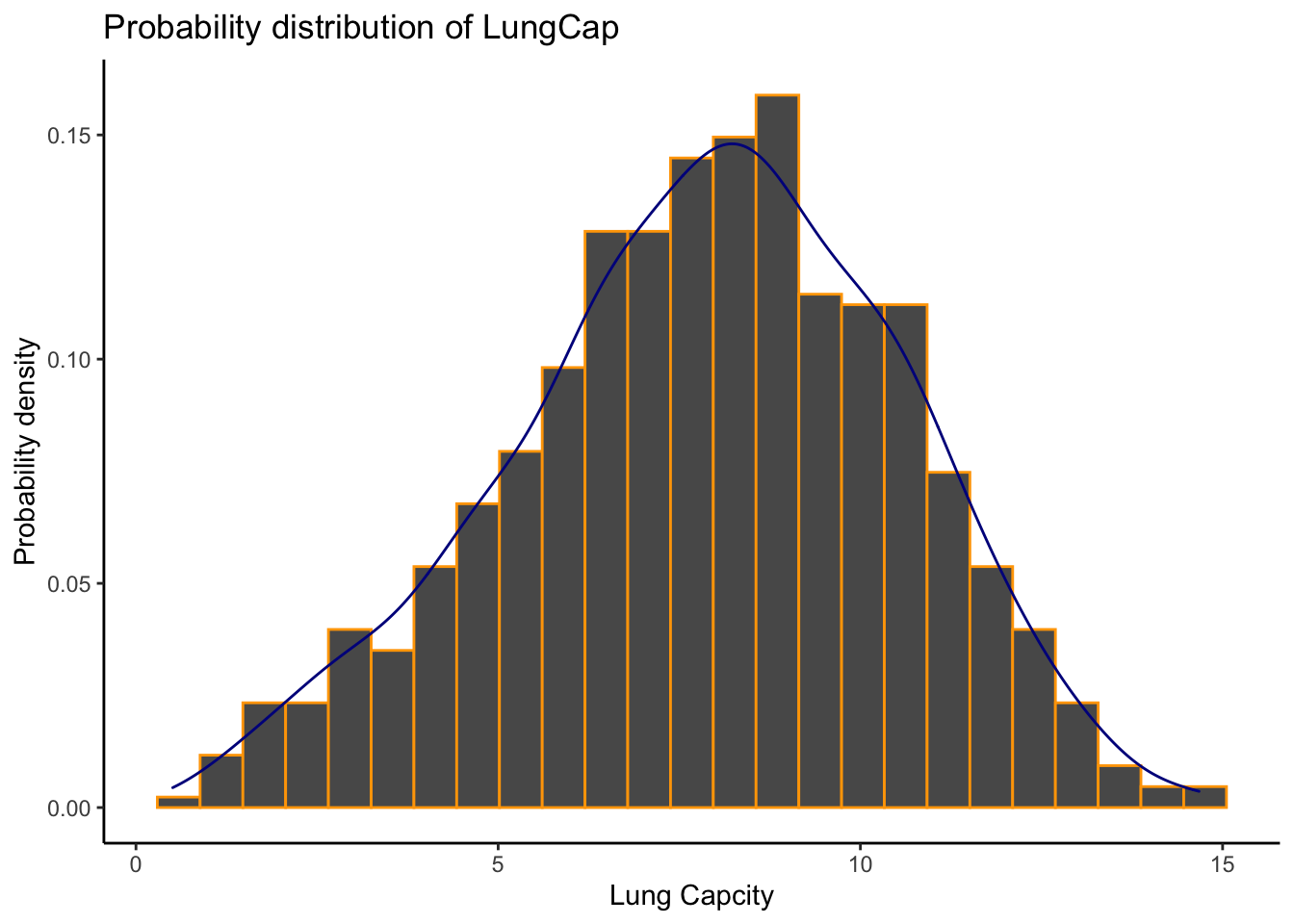
The distribution of LungCap looks as follows:

The histogram and density plots show that it is pretty close to a normal distribution. Most of the observations are close to the mean.
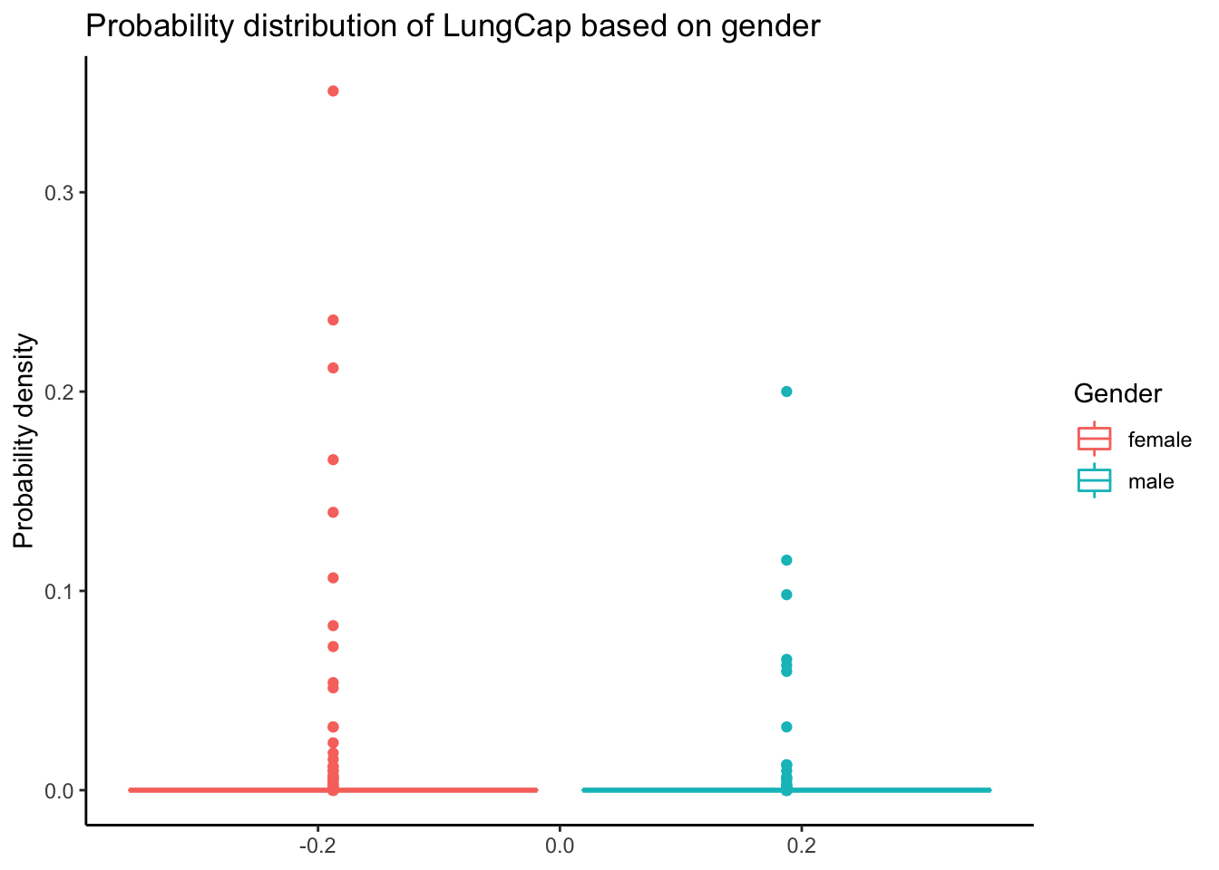
The distribution of LungCap on basis of gender looks as follows:

The box plot shows that the probability density of the male is lesser than the female.
Comparison of mean lung capacities between smokers and non-smokers:
From the above table, we see that the mean lung capacity of those who smoke is greater than those who don’t smoke, but it doesn’t make sense. It also depends on the biological factors of the person who smoke, so we can’t conclude it.
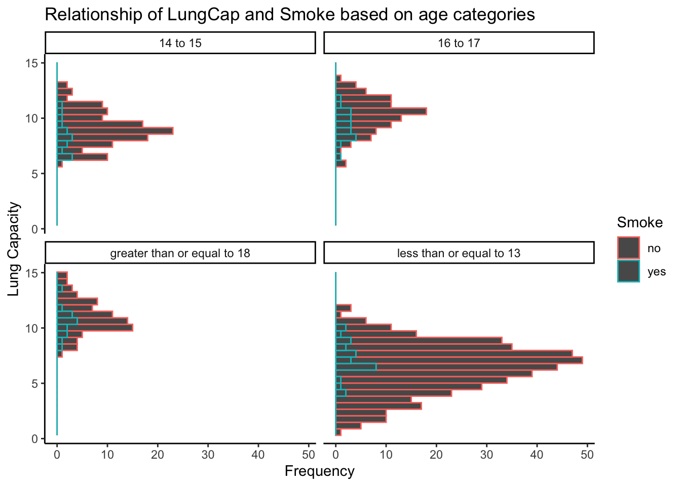
Relationship between Smoke and Lung capacity on basis of given age categories:
Lc <- mutate(Lc, AgeGrp = case_when(Age <= 13 ~ "less than or equal to 13",
Age == 14 | Age == 15 ~ "14 to 15",
Age == 16 | Age == 17 ~ "16 to 17",
Age >= 18 ~ "greater than or equal to 18"))
Lc %>%
ggplot(aes(y = LungCap, color = Smoke)) +
geom_histogram(bins = 25) +
facet_wrap(vars(AgeGrp)) +
theme_classic() +
labs(title = "Relationship of LungCap and Smoke based on age categories", y = "Lung Capacity", x = "Frequency")
From the above plot, we can derive two important observations: 1. The lung capacity of non smokers is more than smokers. 2. The people who smoke are less in age group of “less than or equal to 13”. So as the result as age increases the lung capacity decreases.
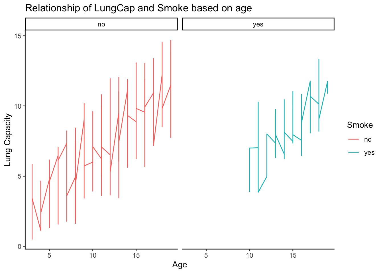
Relationship between Smoke and Lung capacity on basis of age:

Form the above data we can compare 1d and 1e and can say the results are pretty similar. Only 10 and above age group smoke.
Calculating the correlation and covariance between Lung Capacity and Age:
[1] 8.738289[1] 0.8196749We can observe from the comparison that the covariance is positive and it indicates that there is a direct relationship between age and lung capacity. And the correlation is also positive, so they move in same direction. We can say from these results that as the age increases, the lung capacity also increases that is they are directly proportional to each other.
Warning: `data_frame()` was deprecated in tibble 1.1.0.
Please use `tibble()` instead.Probability that a randomly selected inmate has exactly 2 prior convictions:
Probability that a randomly selected inmate has fewer than 2 convictions:
Probability that a randomly selected inmate has 2 or fewer prior convictions:
Probability that a randomly selected inmate has more than 2 prior convictions:
Expected value for the number of prior convictions:
Variance for the Prior Convictions:
standard deviation for the Prior Convictions:
---
title: "Homework 1"
author: "Mani Shanker Kamarapu"
description: "The first homework on descriptive statistics and probability"
date: "10/2/2022"
format:
html:
df-print: paged
css: styles.css
toc: true
code-fold: true
code-copy: true
code-tools: true
categories:
- hw1
- desriptive statistics
- probability
---
```{r}
#| label: setup
#| warning: false
library(tidyverse)
library(readxl)
library(ggplot2)
library(stats)
knitr::opts_chunk$set(echo = TRUE)
```
## Question 1
## Reading data
```{r}
Lc <- read_excel("_data/LungCapData.xls")
Lc
```
The data consists of 725 rows and 6 columns. It determines the lung capacity of the based on their age, height and different characteristics. The main key classification that I can see is if they smoke or not.
## 1a
The distribution of LungCap looks as follows:
```{r}
Lc %>%
  ggplot(aes(LungCap, ..density..)) +
  geom_histogram(bins= 25, color = "orange") +
  geom_density(color = "darkblue") +
  theme_classic() +
  labs(title = "Probability distribution of LungCap", x = "Lung Capcity", y = "Probability density")
```
The histogram and density plots show that it is pretty close to a normal distribution. Most of the observations are close to the mean.
## 1b
The distribution of LungCap on basis of gender looks as follows:
```{r}
Lc %>%
  ggplot(aes(y = dnorm(LungCap), color = Gender)) +
  geom_boxplot() +
  theme_classic() +
  labs(title = "Probability distribution of LungCap based on gender", y = "Probability density")
```
The box plot shows that the probability density of the male is lesser than the female.
## 1c
Comparison of mean lung capacities between smokers and non-smokers:
```{r}
Mean_smoke <- Lc %>%
  group_by(Smoke) %>%
  summarise(mean = mean(LungCap))
Mean_smoke
```
From the above table, we see that the mean lung capacity of those who smoke is greater than those who don't smoke, but it doesn't make sense. It also depends on the biological factors of the person who smoke, so we can't conclude it.
## 1d
Relationship between Smoke and Lung capacity on basis of given age categories:
```{r}
Lc <- mutate(Lc, AgeGrp = case_when(Age <= 13 ~ "less than or equal to 13",
                                    Age == 14 | Age == 15 ~ "14 to 15",
                                    Age == 16 | Age == 17 ~ "16 to 17",
                                    Age >= 18 ~ "greater than or equal to 18"))

Lc %>%
  ggplot(aes(y = LungCap, color = Smoke)) +
  geom_histogram(bins = 25) +
  facet_wrap(vars(AgeGrp)) +
  theme_classic() +
  labs(title = "Relationship of LungCap and Smoke based on age categories", y = "Lung Capacity", x = "Frequency")
```
From the above plot, we can derive two important observations:
1. The lung capacity of non smokers is more than smokers.
2. The people who smoke are less in age group of "less than or equal to 13".
So as the result as age increases the lung capacity decreases.
## 1e
Relationship between Smoke and Lung capacity on basis of age:
```{r}
Lc %>%
  ggplot(aes(x = Age, y = LungCap, color = Smoke)) +
  geom_line() +
  theme_classic() +
  facet_wrap(vars(Smoke)) +
  labs(title = "Relationship of LungCap and Smoke based on age", y = "Lung Capacity", x = "Age")
```
Form the above data we can compare 1d and 1e and can say the results are pretty similar. Only 10 and above age group smoke.
## 1f
Calculating the correlation and covariance between Lung Capacity and Age:
```{r}
Covariance <- cov(Lc$LungCap, Lc$Age)
Correlation <- cor(Lc$LungCap, Lc$Age)
Covariance
Correlation
```
We can observe from the comparison that the covariance is positive and it indicates that there is a direct relationship between age and lung capacity. And the correlation is also positive, so they move in same direction. We can say from these results that as the age increases, the lung capacity also increases that is they are directly proportional to each other.
## Question 2
## Reading the table
```{r}
Prior_convitions <- c(0:4)
Inmate_count <- c(128, 434, 160, 64, 24)
Pc <- data_frame(Prior_convitions, Inmate_count)
Pc
```
```{r}
Pc <- mutate(Pc, Probability = Inmate_count/sum(Inmate_count))
Pc
```
## 2a
Probability that a randomly selected inmate has exactly 2 prior convictions:
```{r}
Pc %>%
  filter(Prior_convitions == 2) %>%
  select(Probability)
```
## 2b
Probability that a randomly selected inmate has fewer than 2 convictions:
```{r}
temp <- Pc %>%
  filter(Prior_convitions < 2)
sum(temp$Probability)
```
## 2c
Probability that a randomly selected inmate has 2 or fewer prior convictions:
```{r}
temp <- Pc %>%
  filter(Prior_convitions <= 2)
sum(temp$Probability)
```
## 2d
Probability that a randomly selected inmate has more than 2 prior convictions:
```{r}
temp <- Pc %>%
  filter(Prior_convitions > 2)
sum(temp$Probability)
```
## 2e
Expected value for the number of prior convictions:
```{r}
Pc <- mutate(Pc, Wm = Prior_convitions*Probability)
e <- sum(Pc$Wm)
e
```
## 2f
Variance for the Prior Convictions:
```{r}
v <-sum(((Pc$Prior_convitions-e)^2)*Pc$Probability)
v
```
standard deviation for the Prior Convictions:
```{r}
sqrt(v)
```