Homework 5

library(tidyverse)
library(alr4)
library(smss)

knitr::opts_chunk$set(echo = TRUE, warning = FALSE, message = FALSE)

Qn 1A

Beds, as it has the largest p-value.

Qn 1B

Size, as it would produce the smallest p-value.

Qn 1C

Beds is highly correlated with Size, so multicollinearity might be a possible reason for this.

Qn 1D

The model with all predictors has the highest R².

data(house.selling.price.2)
summary(lm(P ~ ., house.selling.price.2))

Call:
lm(formula = P ~ ., data = house.selling.price.2)

Residuals:
    Min      1Q  Median      3Q     Max 
-36.212  -9.546   1.277   9.406  71.953 

Coefficients:
            Estimate Std. Error t value Pr(>|t|)    
(Intercept)  -41.795     12.104  -3.453 0.000855 ***
S             64.761      5.630  11.504  < 2e-16 ***
Be            -2.766      3.960  -0.698 0.486763    
Ba            19.203      5.650   3.399 0.001019 ** 
New           18.984      3.873   4.902  4.3e-06 ***
---
Signif. codes:  0 '***' 0.001 '**' 0.01 '*' 0.05 '.' 0.1 ' ' 1

Residual standard error: 16.36 on 88 degrees of freedom
Multiple R-squared:  0.8689,    Adjusted R-squared:  0.8629 
F-statistic: 145.8 on 4 and 88 DF,  p-value: < 2.2e-16

The model below without Beds has the highest adjusted R² and lowest PRESS/BIC/AIC.

model <- lm(P ~ .-Be, house.selling.price.2)

PRESS <- function(model) {
  pr <- residuals(model)/(1-lm.influence(model)$hat)
  PRESS <- sum(pr^2)
  return(PRESS)
}

PRESS(model)

[1] 27860.05

BIC(model)

[1] 801.7996

AIC(model)

[1] 789.1366

Qn 1E

I prefer the model without Beds because it doesn’t seem to be adding great value to the regression model, and the other 4 measures (adjusted R², PRESS, AIC and BIC) are better ways of assessing a multiple regression model than just R².

Qn 2A

data(trees)
model2 <- lm(Volume ~ poly(Girth, 2) + Height, trees)
summary(model2)

Call:
lm(formula = Volume ~ poly(Girth, 2) + Height, data = trees)

Residuals:
    Min      1Q  Median      3Q     Max 
-4.2928 -1.6693 -0.1018  1.7851  4.3489 

Coefficients:
                Estimate Std. Error t value Pr(>|t|)    
(Intercept)      1.56553    6.72218   0.233 0.817603    
poly(Girth, 2)1 80.25223    3.07346  26.111  < 2e-16 ***
poly(Girth, 2)2 15.39923    2.63157   5.852 3.13e-06 ***
Height           0.37639    0.08823   4.266 0.000218 ***
---
Signif. codes:  0 '***' 0.001 '**' 0.01 '*' 0.05 '.' 0.1 ' ' 1

Residual standard error: 2.625 on 27 degrees of freedom
Multiple R-squared:  0.9771,    Adjusted R-squared:  0.9745 
F-statistic: 383.2 on 3 and 27 DF,  p-value: < 2.2e-16

Qn 2B

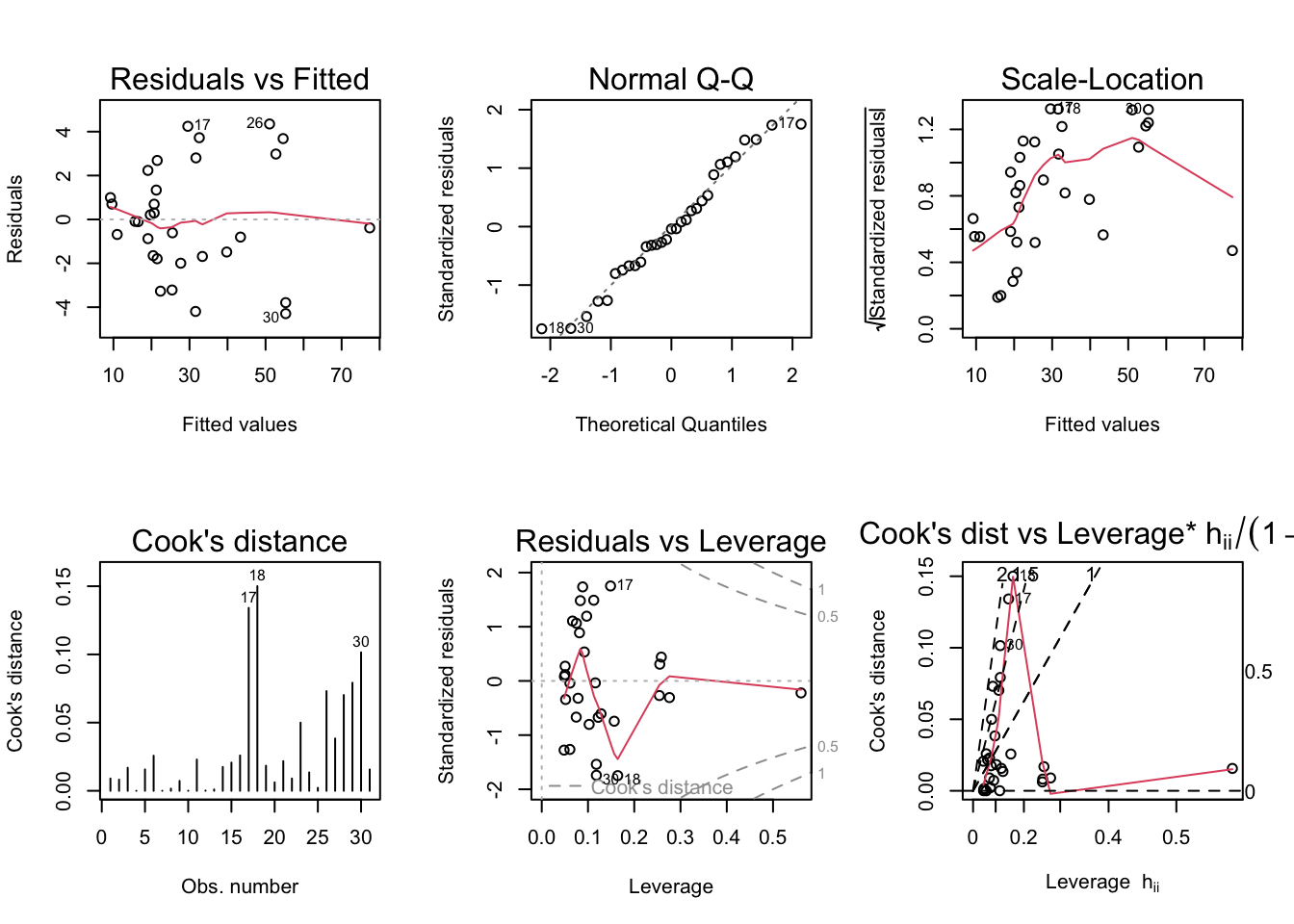
par(mfrow = c(2,3)); plot(model2, which = 1:6)

Scale-Location plot indicates heteroskedasticity. Cook’s distance, residuals vs. leverage and Cook’s distance vs. leverage plots indicate 3 outliers.

Qn 3A

data(florida)
model3a <- lm(Buchanan ~ Bush, florida)
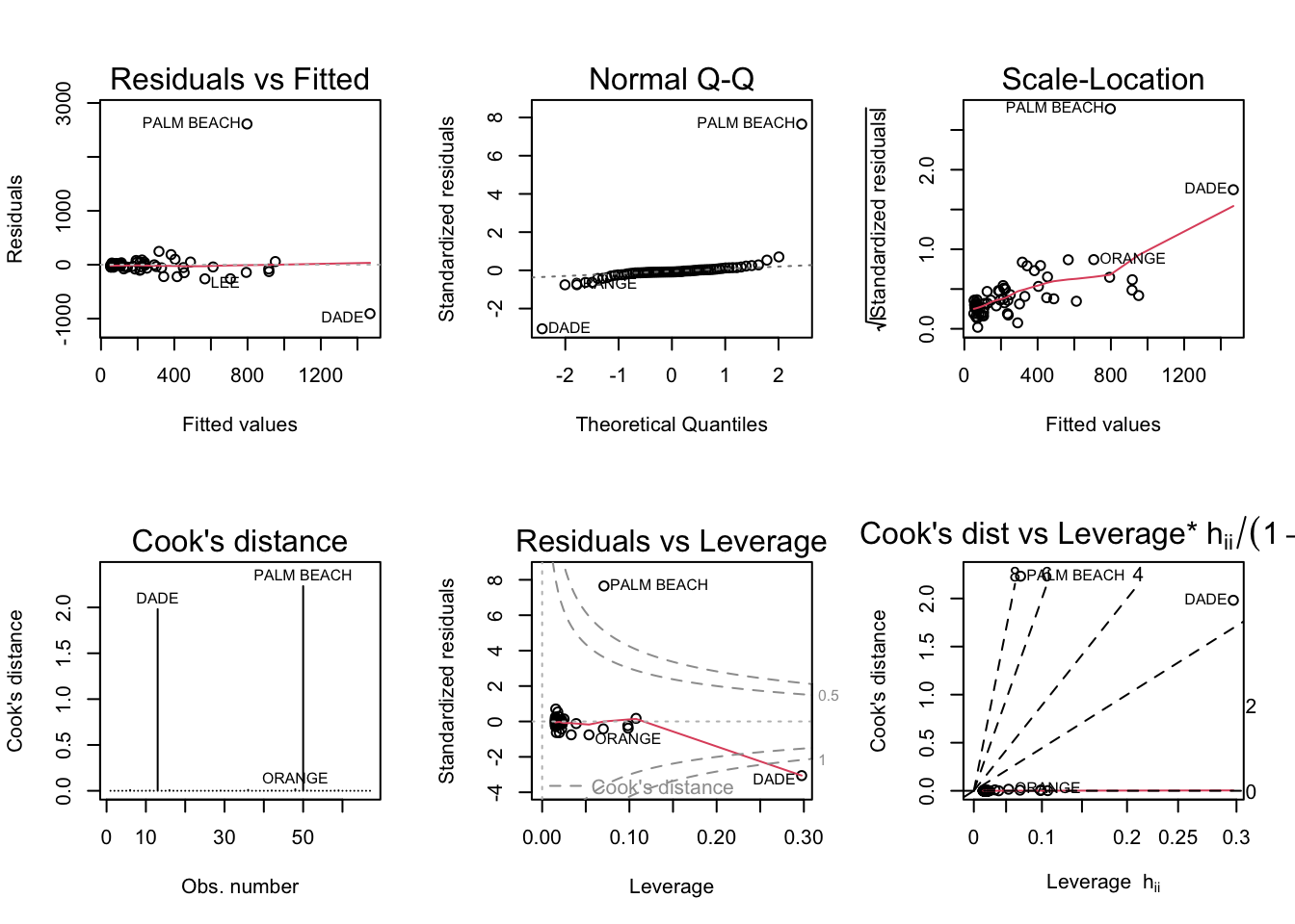
par(mfrow = c(2,3)); plot(model3a, which = 1:6)

It seems to stick out in all 6 plots, so I would say it’s an outlier.

Qn 3B

model3b <- lm(log(Buchanan) ~ log(Bush), florida)
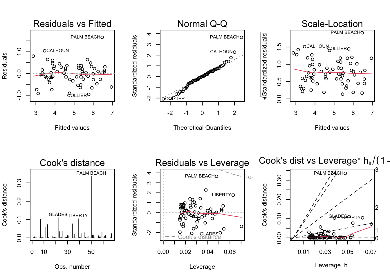
par(mfrow = c(2,3)); plot(model3b, which = 1:6)

Palm Beach still seems to be an outlier, but the diagnostic plots look more normal than in the previous model.