Code
library(tidyverse)
library(readxl)
library(ggplot2)
library(stats)

knitr::opts_chunk$set(echo = TRUE)Mani Kanta Gogula
October 3, 2022
Given data consists of 725 rows and 6 columns
`stat_bin()` using `bins = 30`. Pick better value with `binwidth`.
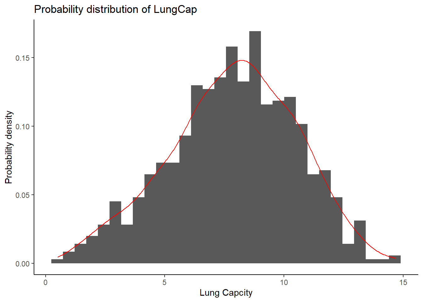
Based on above histogram , we can say the distribution is very close to the normal distribution
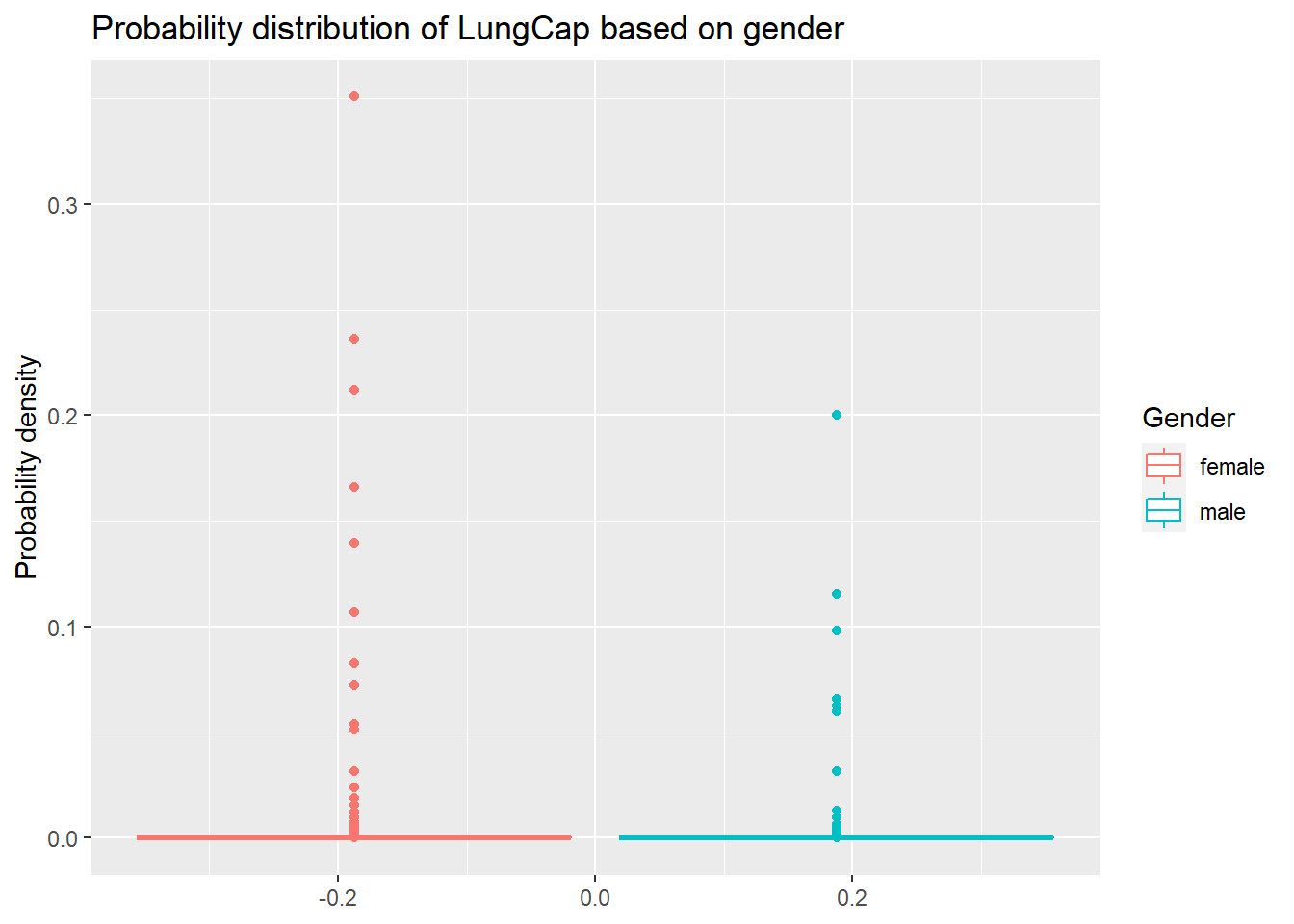
Compare the probability distribution of the LungCap with respect to Males and Females?

Compare the mean lung capacities for smokers and non-smokers. Does it make sense?
The mean of the lung capacity who smokes is greater than the people who doesnt smoke which doesnt make any sense in practical
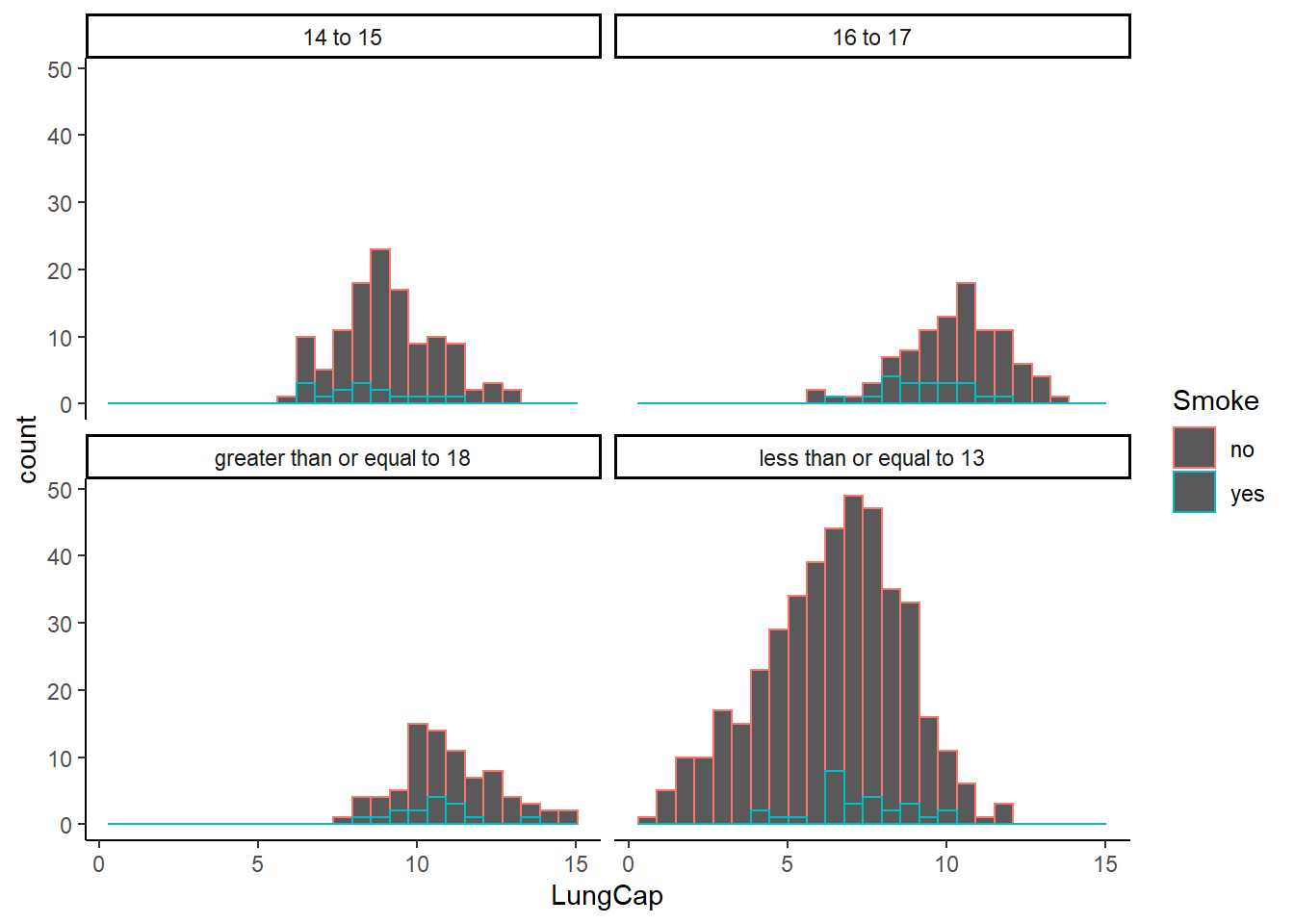
Examine the relationship between Smoking and Lung Capacity within age groups: “less than or equal to 13”, “14 to 15”, “16 to 17”, and “greater than or equal to 18”.
Lung_data <- mutate(Lung_data, AgeGrp = case_when(Age <= 13 ~ "less than or equal to 13",
Age == 14 | Age == 15 ~ "14 to 15",
Age == 16 | Age == 17 ~ "16 to 17",
Age >= 18 ~ "greater than or equal to 18"))
Lung_data %>%
ggplot(aes(y = LungCap, color = Smoke)) +
geom_histogram(bins = 25) +
facet_wrap(vars(AgeGrp)) +
theme_classic() + coord_flip()
$y
[1] "Lung Capacity"
$x
[1] "Frequency"
$title
[1] "Relationship of LungCap and Smoke based on age categories"
attr(,"class")
[1] "labels"Compare the lung capacities for smokers and non-smokers within each age group. Is your answer different from the one in part d. What could possibly be going on here?

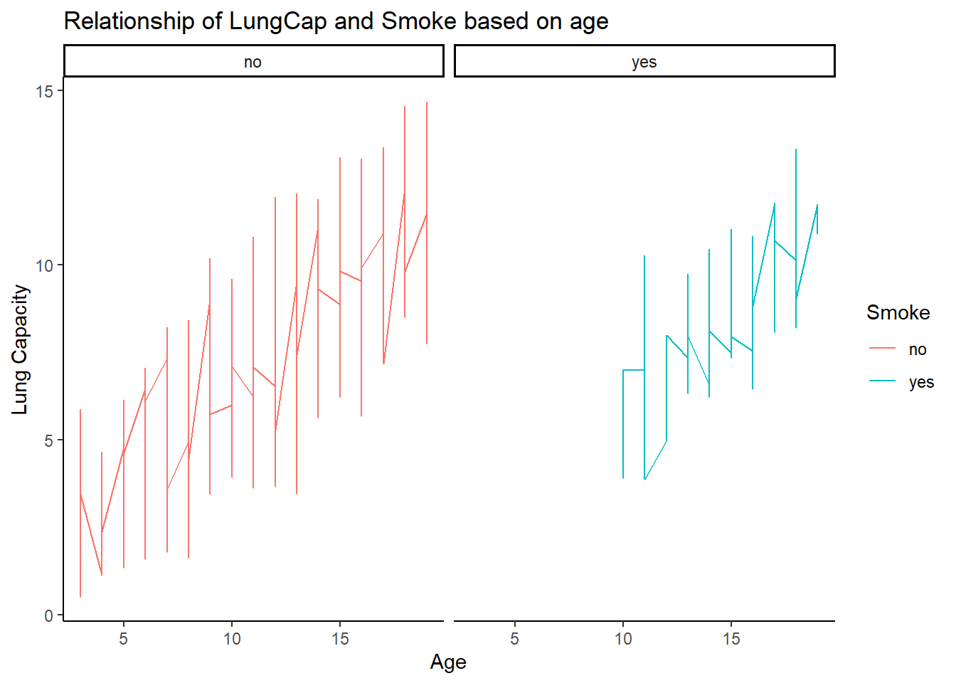
Form the above data we can compare 1d and 1e and can say the results are pretty similar. Only 10 and above age group smoke.
Calculate the correlation and covariance between Lung Capacity and Age. (use the cov() and cor() functions in R). Interpret your results.
[1] 8.738289[1] 0.8196749From the above result we can say that both covariance and correlation is positive and which indicates direct relationship that means Lungcapacity increases as age increases
Warning: `data_frame()` was deprecated in tibble 1.1.0.
Please use `tibble()` instead.
This warning is displayed once every 8 hours.
Call `lifecycle::last_lifecycle_warnings()` to see where this warning was generated.What is the probability that a randomly selected inmate has exactly 2 prior convictions?
What is the probability that a randomly selected inmate has fewer than 2 prior convictions?
What is the probability that a randomly selected inmate has 2 or fewer prior convictions?
What is the probability that a randomly selected inmate has more than 2 prior convictions?
What is the expected value for the number of prior convictions?
Calculate the variance and the standard deviation for the Prior Convictions.
standard deviation:
---
title: "Homework 1"
author: "Mani Kanta Gogula"
description: "Homework_1_603"
date: "10/3/2022"
format:
html:
df-print: paged
css: styles.css
toc: true
code-fold: true
code-copy: true
code-tools: true
categories:
- hw1
- desriptive statistics
- probability
---
```{r}
#| label: setup
#| warning: false
library(tidyverse)
library(readxl)
library(ggplot2)
library(stats)
knitr::opts_chunk$set(echo = TRUE)
```
## Question 1
```{r}
Lung_data<- read_excel("C:/Users/manik/Desktop/LungCapData.xls")
Lung_data
```
Given data consists of 725 rows and 6 columns
a. What does the distribution of LungCap look like?
```{r}
Lung_data %>%
  ggplot(aes(LungCap, ..density..)) +
  geom_histogram() +
  geom_density(color = "Red") +
  theme_classic() +
  labs(title = "Probability distribution of LungCap", x = "Lung Capcity", y = "Probability density")
```
Based on above histogram , we can say the distribution is very close to the normal distribution
Compare the probability distribution of the LungCap with respect to Males and
Females?
```{r}
Lung_data %>%
  ggplot(aes(y = dnorm(LungCap), color = Gender)) +
  geom_boxplot() +
  labs(title = "Probability distribution of LungCap based on gender", y = "Probability density")
```
Compare the mean lung capacities for smokers and non-smokers. Does it make
sense?
```{r}
Mean_smokers <- Lung_data %>%
  group_by(Smoke) %>%
  summarise(mean = mean(LungCap))
Mean_smokers
```
The mean of the lung capacity who smokes is greater than the people who doesnt smoke which doesnt make any sense in practical
Examine the relationship between Smoking and Lung Capacity within age
groups: “less than or equal to 13”, “14 to 15”, “16 to 17”, and “greater than or
equal to 18”.
```{r}
Lung_data <- mutate(Lung_data, AgeGrp = case_when(Age <= 13 ~ "less than or equal to 13",
                                    Age == 14 | Age == 15 ~ "14 to 15",
                                    Age == 16 | Age == 17 ~ "16 to 17",
                                    Age >= 18 ~ "greater than or equal to 18"))

Lung_data %>%
  ggplot(aes(y = LungCap, color = Smoke)) +
  geom_histogram(bins = 25) +
  facet_wrap(vars(AgeGrp)) +
  theme_classic() + coord_flip()
labs(title = "Relationship of LungCap and Smoke based on age categories", y = "Lung Capacity", x = "Frequency")
```
Compare the lung capacities for smokers and non-smokers within each age
group. Is your answer different from the one in part d. What could possibly be
going on here?
```{r}
Lung_data %>%
  ggplot(aes(x = Age, y = LungCap, color = Smoke)) +
  geom_line() +
  theme_classic() +
  facet_wrap(vars(Smoke)) +
  labs(title = "Relationship of LungCap and Smoke based on age", y = "Lung Capacity", x = "Age")
```
Form the above data we can compare 1d and 1e and can say the results are pretty similar. Only 10 and above age group smoke.
Calculate the correlation and covariance between Lung Capacity and Age. (use
the cov() and cor() functions in R). Interpret your results.
```{r}
Covariance_LA <- cov(Lung_data$LungCap, Lung_data$Age)
Correlation_LA <- cor(Lung_data$LungCap, Lung_data$Age)
Covariance_LA
Correlation_LA
```
From the above result we can say that both covariance and correlation is positive and which indicates direct relationship that means Lungcapacity increases as age increases
## Question 2
```{r}
Prior_convitions <- c(0:4)
Inmate_count <- c(128, 434, 160, 64, 24)
IP<- data_frame(Prior_convitions, Inmate_count)
IP
```
```{r}
IP <- mutate(IP, Probability = Inmate_count/sum(Inmate_count))
IP
```
What is the probability that a randomly selected inmate has exactly 2 prior
convictions?
```{r}
IP %>%
  filter(Prior_convitions == 2) %>%
  select(Probability)
```
What is the probability that a randomly selected inmate has fewer than 2 prior
convictions?
```{r}
p_2 <- IP %>%
  filter(Prior_convitions < 2)
sum(p_2$Probability)
```
What is the probability that a randomly selected inmate has 2 or fewer prior
convictions?
```{r}
p <- IP %>%
  filter(Prior_convitions <= 2)
sum(p$Probability)
```
What is the probability that a randomly selected inmate has more than 2 prior
convictions?
```{r}
P_3 <- IP %>%
  filter(Prior_convitions > 2)
sum(P_3$Probability)
```
What is the expected value for the number of prior convictions?
```{r}
IP <- mutate(IP, Wm = Prior_convitions*Probability)
expe<- sum(IP$Wm)
expe
```
Calculate the variance and the standard deviation for the Prior Convictions.
```{r}
var_ <-sum(((IP$Prior_convitions-expe)^2)*IP$Probability)
var_
```
standard deviation:
```{r}
sqrt(var_)
```