Code
library(tidyverse)
library(readxl)

knitr::opts_chunk$set(echo = TRUE)Quinn He
October 3, 2022
`stat_bin()` using `bins = 30`. Pick better value with `binwidth`.

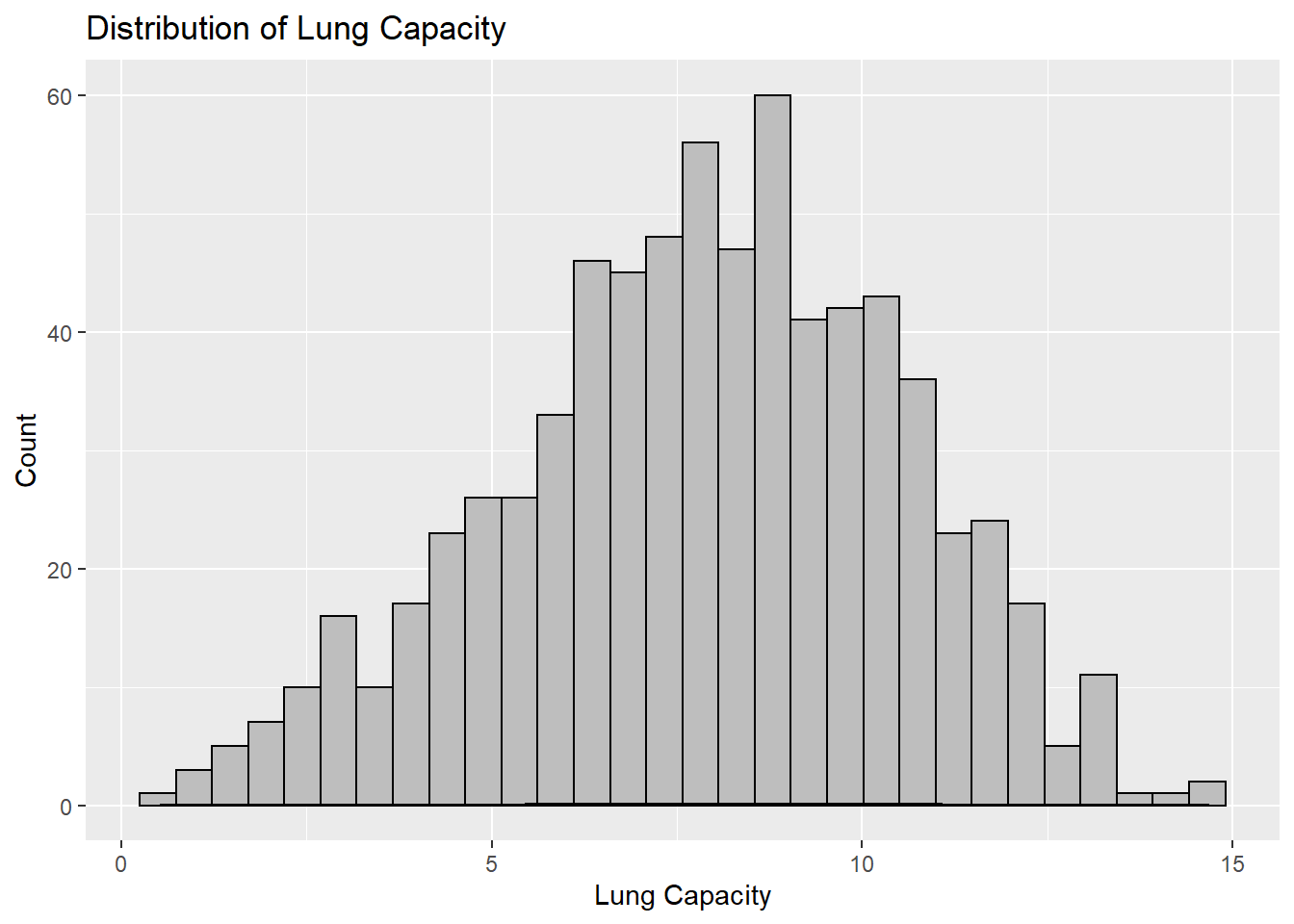
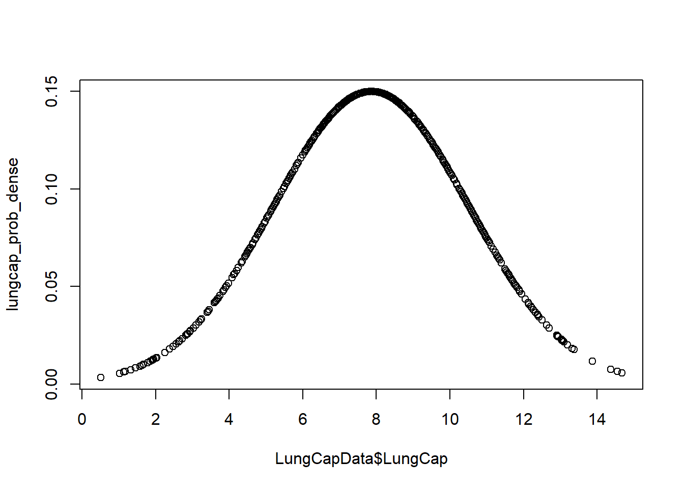
With these two functions I can see the distribution is normal with both a histogram and regular graph. The second graph more clearly depicts a normal distribution with the probability density points laid throughout. ## 1b
It looks like men, on average, have a higher lung capacity than females, but only by a slim margin. Overall, lung capacity is relatively similar among genders. The real comparison will come with smokers and nonsmokers. ## 1c
# A tibble: 2 × 2
Smoke lung_cap_mean
<chr> <dbl>
1 no 7.77
2 yes 8.65Above is the lung capacity mean for smokers and nonsmokers. I’m actually a little surprised the mean lung capacity for nonsmokers is slightly higher than that of nonsmokers. I would think the opposite to be true, but I suspect because there is a range of ages under 18 and the body is not fully developed yet, I imagine a 6 year old nonsmoker will not have the same lung capacity as a 17 year old smoker.
Below I created a bunch of variables to separate people into certain age groups. I imagine there would be an easier way to separate them.
#LungCapData %>%
#group_by(Age) %>%
#summarise(lungcap = mean(LungCap))
age13 <- LungCapData %>%
filter(Age <= 13) %>%
group_by(Smoke) %>%
summarise(lung_cap_mean = mean(LungCap))
age1415 <- LungCapData %>%
filter(Age == 14 | Age == 15) %>%
group_by(Smoke) %>%
summarise(lung_cap_mean = mean(LungCap))
age1617 <- LungCapData %>%
filter(Age == 16 | Age == 17) %>%
group_by(Smoke) %>%
summarise(lung_cap_mean = mean(LungCap))
age18 <- LungCapData %>%
filter(Age >= 18) %>%
group_by(Smoke) %>%
summarise(lung_cap_mean = mean(LungCap))
age13# A tibble: 2 × 2
Smoke lung_cap_mean
<chr> <dbl>
1 no 6.36
2 yes 7.20# A tibble: 2 × 2
Smoke lung_cap_mean
<chr> <dbl>
1 no 9.14
2 yes 8.39# A tibble: 2 × 2
Smoke lung_cap_mean
<chr> <dbl>
1 no 10.5
2 yes 9.38# A tibble: 2 × 2
Smoke lung_cap_mean
<chr> <dbl>
1 no 11.1
2 yes 10.5Based on the variables I created above, it appears the lung capacity for people under 13, and that smoke, is higher than people who do not smoke. As the age brackets increase, so does lung capacity overall, but it begins to show that those who do smoke, generally have a lower lung capacity than those who choose not to smoke. This is what I would expect to happen since a 13 year old still has plenty of growing to do, therefore the lung capacity will be much lower than a grown teenager.
With a correlation of 0.81, lung capacity and age have a fairly strong positive relationship. This is what I figured would be the case. As people age, their lung capacities grow larger. A 17 year old will be more developed and most likely have a larger lung capacity than, say, a child the age of 8.
I created a table of the data frame in question 2
The probability of selecting inmates with 2 prior convictions is 19.7%.
The probability of selecting inmates with less than 2 prior convictions is 69%.
The probability of selecting inmates with 2 or less prior convictions is 89%.
The probability of selecting inmates with more than 2 prior convictions is 10.8%.
The expected value for number of prior convictions is 291.4.
use rep()
---
title: "Homework 1"
author: "Quinn He"
desription: "Homework 1"
date: "10/03/2022"
format:
html:
toc: true
code-fold: true
code-copy: true
code-tools: true
categories:
- hw1
---
```{r}
#| label: setup
#| warning: false
library(tidyverse)
library(readxl)
knitr::opts_chunk$set(echo = TRUE)
```
### Reading in the data
```{r}
LungCapData <- read_excel("_data/LungCapData.xls")

lungcap_prob_dense <- dnorm(LungCapData$LungCap, mean = 7.863, sd = 2.662)
```
## 1a
```{r}
ggplot(LungCapData, mapping = aes(LungCap)) +
  geom_histogram(color = "black", fill = "grey")+
  geom_density()+
  labs(title = "Distribution of Lung Capacity", x = "Lung Capacity", y = "Count")
plot(x = LungCapData$LungCap, y = lungcap_prob_dense)
```
With these two functions I can see the distribution is normal with both a histogram and regular graph. The second graph more clearly depicts a normal distribution with the probability density points laid throughout.
## 1b
```{r}
ggplot(LungCapData, mapping = aes(x = Gender, y = LungCap)) +
  geom_boxplot()
```
It looks like men, on average, have a higher lung capacity than females, but only by a slim margin. Overall, lung capacity is relatively similar among genders. The real comparison will come with smokers and nonsmokers.
## 1c
```{r}
LungCapData %>%
  group_by(Smoke) %>%
  summarise(lung_cap_mean = mean(LungCap))
```
Above is the lung capacity mean for smokers and nonsmokers. I'm actually a little surprised the mean lung capacity for nonsmokers is slightly higher than that of nonsmokers. I would think the opposite to be true, but I suspect because there is a range of ages under 18 and the body is not fully developed yet, I imagine a 6 year old nonsmoker will not have the same lung capacity as a 17 year old smoker.
## 1d
Below I created a bunch of variables to separate people into certain age groups. I imagine there would be an easier way to separate them.
```{r}
#LungCapData %>%
  #group_by(Age) %>%
  #summarise(lungcap = mean(LungCap))

age13 <- LungCapData %>%
  filter(Age <= 13) %>%
  group_by(Smoke) %>%
  summarise(lung_cap_mean = mean(LungCap))

age1415 <- LungCapData %>%
  filter(Age == 14 | Age == 15) %>%
  group_by(Smoke) %>%
  summarise(lung_cap_mean = mean(LungCap))

age1617 <- LungCapData %>%
  filter(Age == 16 | Age == 17) %>%
  group_by(Smoke) %>%
  summarise(lung_cap_mean = mean(LungCap))

age18 <- LungCapData %>%
  filter(Age >= 18) %>%
  group_by(Smoke) %>%
  summarise(lung_cap_mean = mean(LungCap))

age13
age1415
age1617
age18
```
## 1e
Based on the variables I created above, it appears the lung capacity for people under 13, and that smoke, is higher than people who do not smoke. As the age brackets increase, so does lung capacity overall, but it begins to show that those who do smoke, generally have a lower lung capacity than those who choose not to smoke. This is what I would expect to happen since a 13 year old still has plenty of growing to do, therefore the lung capacity will be much lower than a grown teenager.
## 1f
```{r}
cor(LungCapData$LungCap, LungCapData$Age)
```
With a correlation of 0.81, lung capacity and age have a fairly strong positive relationship. This is what I figured would be the case. As people age, their lung capacities grow larger. A 17 year old will be more developed and most likely have a larger lung capacity than, say, a child the age of 8.
I created a table of the data frame in question 2
```{r}
xx <- c(0:4)

freq <- c(128, 434, 160, 64, 24)

df <- tibble(xx, freq)
```
## 2a
```{r}
160/810
```
The probability of selecting inmates with 2 prior convictions is 19.7%.
## 2b
```{r}
562/810
```
The probability of selecting inmates with less than 2 prior convictions is 69%.
## 2c
```{r}
722/810
```
The probability of selecting inmates with 2 or less prior convictions is 89%.
## 2d
```{r}
88/810
```
The probability of selecting inmates with more than 2 prior convictions is 10.8%.
## 2e
The expected value for number of prior convictions is 291.4.
```{r}
test <- c(128, 434, 160, 64, 24)

testprobs <- c(0.15, 0.54, 0.2, 0.08, 0.03)

sum(test*testprobs)
```
## 2f
use rep()
```{r}
convictions <- c(rep(0,128), rep(1, 434), rep(2,160), rep(3,64), rep(4,24))

sd(convictions)
var(convictions)
```