Homework 3

hw3

Mani Kanta Gogula

Home work 3

Author

Mani Kanta

Published

November 11, 2022

Code

library(tidyverse)
library(ggplot2)
library(stats)
library(alr4)
library(smss)

knitr::opts_chunk$set(echo = TRUE)

Question 1

Code

data(UN11)
UN11

A

The Predicted variable here is ppgdp.

B

Code

UN11 %>%
  select(c(ppgdp,fertility)) %>%
  ggplot(aes(x = ppgdp, y = fertility)) + 
  geom_point()+
  geom_smooth(method=lm)

`geom_smooth()` using formula 'y ~ x'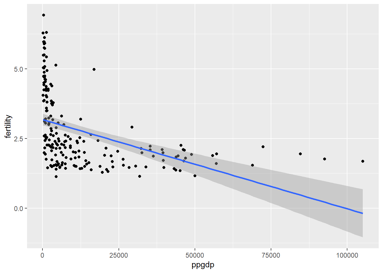

The graph show negative realtionship between ppgdp and fertility and here straight line mean function does not seem an appropriate measure for a summary of this graph.

C

Code

UN11 %>%
  select(c(ppgdp,fertility)) %>%
  ggplot(aes(x = log(ppgdp), y = log(fertility))) + 
  geom_point()+
  geom_smooth(method=lm)

`geom_smooth()` using formula 'y ~ x'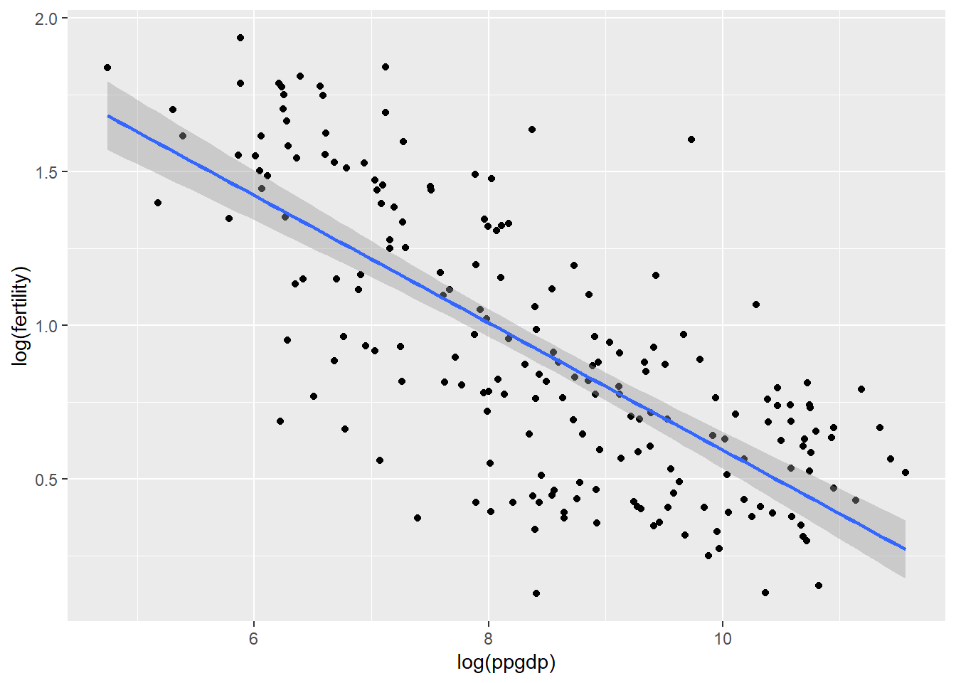

The relationship between the variables appears to be negative throughout the graph. The simple linear regression seems plausible for summary of this graph.

Question 2

A

Code

UN11$british <- 1.33 * UN11$ppgdp
summary(lm(fertility ~ british, UN11))


Call:
lm(formula = fertility ~ british, data = UN11)

Residuals:
    Min      1Q  Median      3Q     Max 
-1.9006 -0.8801 -0.3547  0.6749  3.7585 

Coefficients:
              Estimate Std. Error t value Pr(>|t|)    
(Intercept)  3.178e+00  1.048e-01  30.331  < 2e-16 ***
british     -2.407e-05  3.500e-06  -6.877  7.9e-11 ***
---
Signif. codes:  0 '***' 0.001 '**' 0.01 '*' 0.05 '.' 0.1 ' ' 1

Residual standard error: 1.206 on 197 degrees of freedom
Multiple R-squared:  0.1936,    Adjusted R-squared:  0.1895 
F-statistic: 47.29 on 1 and 197 DF,  p-value: 7.903e-11

Code

summary(lm(fertility ~ ppgdp, UN11))


Call:
lm(formula = fertility ~ ppgdp, data = UN11)

Residuals:
    Min      1Q  Median      3Q     Max 
-1.9006 -0.8801 -0.3547  0.6749  3.7585 

Coefficients:
              Estimate Std. Error t value Pr(>|t|)    
(Intercept)  3.178e+00  1.048e-01  30.331  < 2e-16 ***
ppgdp       -3.201e-05  4.655e-06  -6.877  7.9e-11 ***
---
Signif. codes:  0 '***' 0.001 '**' 0.01 '*' 0.05 '.' 0.1 ' ' 1

Residual standard error: 1.206 on 197 degrees of freedom
Multiple R-squared:  0.1936,    Adjusted R-squared:  0.1895 
F-statistic: 47.29 on 1 and 197 DF,  p-value: 7.903e-11

B

Code

cor(UN11$ppgdp, UN11$fertility)

[1] -0.4399891

Code

cor(UN11$british, UN11$fertility)

[1] -0.4399891

There is no change in correlation

Question 3

Code

data(water)
pairs(water)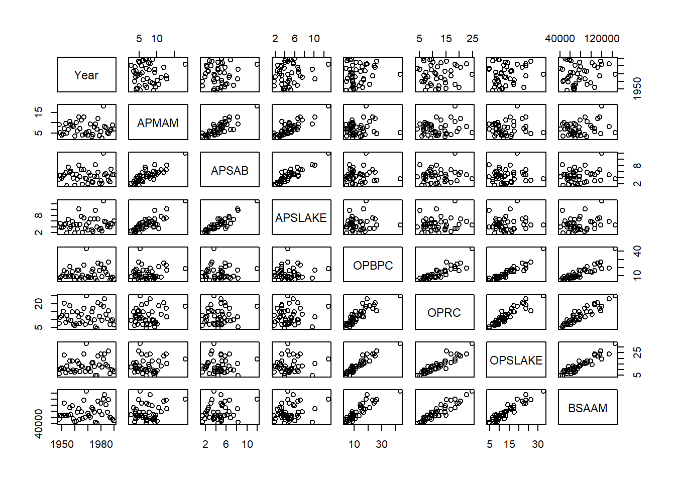

From the above plot, it seems that the stream run-off variable has a relationship to the ‘O’ named lakes but no real notable relationship to the ‘A’ named lakes.

Question 4

Code

data(Rateprof)
rate <- Rateprof %>% select(quality, helpfulness, clarity, easiness, raterInterest)
pairs(rate)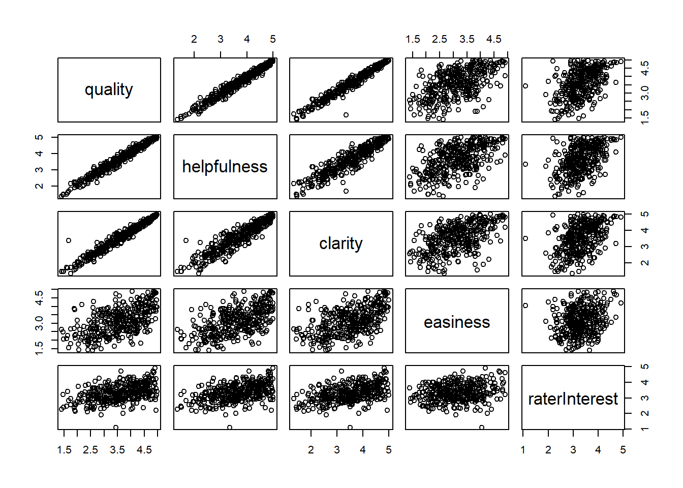

Interpreting to the scatter plot matrix of the average professor ratings for the topics of quality, clarity, helpfulness, easiness, and rater interest, the variables quality, clarity, and helpfulness appear to each have strong positive correlations with each other. The variable easiness appears to have a much weaker positive correlation with helpfulness, clarity, and quality. Rater interest does not appear to have much of a correlation to any of the other variables.So, we can say that Quality, helpfulness and clarity have the clearest linear relationships with one another and Easiness and raterInterest do not seem to have linear relationships with the other variables.

Question 5

Code

data(student.survey)
student.survey

A

Code

student.survey %>%
  select(c(pi, re)) %>%
  ggplot() + 
  geom_bar(aes(x = re, fill = pi)) +
  xlab("Religiosity") +
  ylab("Political ideology")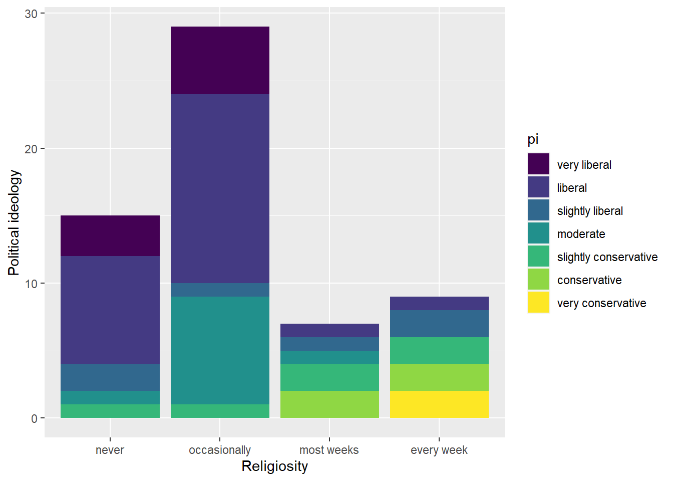

Religiosity and conservatism seem to have a positive relationship.

Code

student.survey %>%
  select(c(tv, hi)) %>%
  ggplot(aes(x = tv, y = hi)) + 
  geom_point() +
  geom_smooth(method=lm) +
  xlab("Average Hours of TV watched per Week") +
  ylab("High School GPA")

`geom_smooth()` using formula 'y ~ x'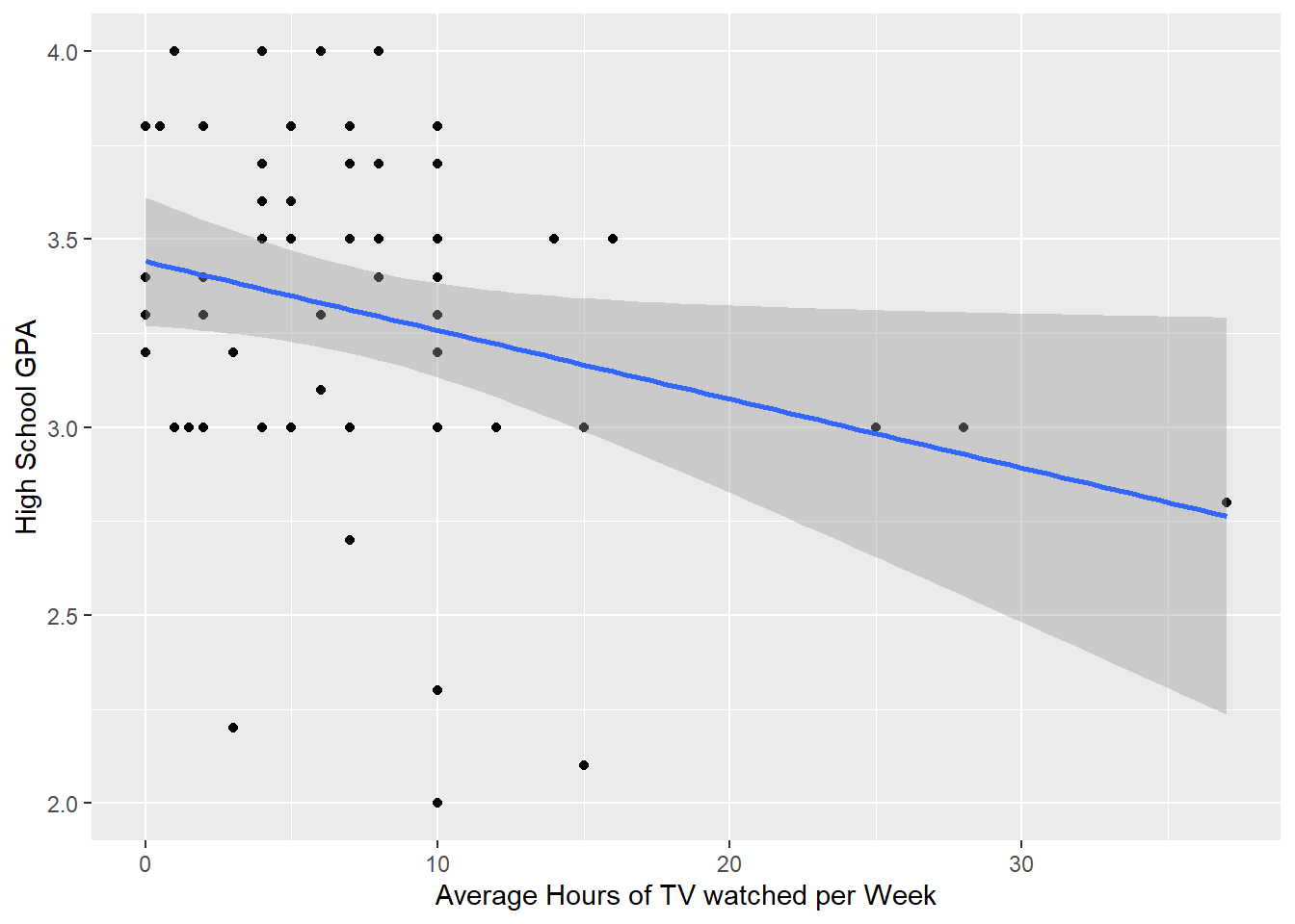

High school GPA and TV-watching seem to have a negative relationship.

B

Code

summary(lm(data = student.survey, formula = as.numeric(pi) ~ as.numeric(re)))


Call:
lm(formula = as.numeric(pi) ~ as.numeric(re), data = student.survey)

Residuals:
     Min       1Q   Median       3Q      Max 
-2.81243 -0.87160  0.09882  1.12840  3.09882 

Coefficients:
               Estimate Std. Error t value Pr(>|t|)    
(Intercept)      0.9308     0.4252   2.189   0.0327 *  
as.numeric(re)   0.9704     0.1792   5.416 1.22e-06 ***
---
Signif. codes:  0 '***' 0.001 '**' 0.01 '*' 0.05 '.' 0.1 ' ' 1

Residual standard error: 1.345 on 58 degrees of freedom
Multiple R-squared:  0.3359,    Adjusted R-squared:  0.3244 
F-statistic: 29.34 on 1 and 58 DF,  p-value: 1.221e-06

At a significance level of 0.01, there is a statistically significant association between religiosity and political ideology (as p-value < .01). The correlation is moderate and positive, suggesting that as weekly church attendance increases, political ideology becomes more conservative leaning.

Code

summary(lm(data = student.survey, formula = hi ~ tv))


Call:
lm(formula = hi ~ tv, data = student.survey)

Residuals:
    Min      1Q  Median      3Q     Max 
-1.2583 -0.2456  0.0417  0.3368  0.7051 

Coefficients:
             Estimate Std. Error t value Pr(>|t|)    
(Intercept)  3.441353   0.085345  40.323   <2e-16 ***
tv          -0.018305   0.008658  -2.114   0.0388 *  
---
Signif. codes:  0 '***' 0.001 '**' 0.01 '*' 0.05 '.' 0.1 ' ' 1

Residual standard error: 0.4467 on 58 degrees of freedom
Multiple R-squared:  0.07156,   Adjusted R-squared:  0.05555 
F-statistic: 4.471 on 1 and 58 DF,  p-value: 0.03879

With a slope of -0.018, there is a negative association between hours of tv watched per week and high school GPA, meaning that as hours of tv viewing increase, a student’s GPA tends to decrease. There is a statistically significant relationship between hours of tv viewed per week and GPA at a significance level of 0.05. However, the R-squared value is close to 0, which suggests that the regression model does not provide a strong prediction for the observed variables. This is not suprising after looking at the scatter plot with hours of tv watched and GPA, since there does not appear to be a linear trend in the data.