Code
library(tidyverse)
library(dplyr)
library(ggplot2)
library(alr4)
library(smss)
knitr::opts_chunk$set(echo = TRUE)Kalimah Muhammad
October 31, 2022
The predictor variable is ppgdp (the gross national product per person in USD) and the response or outcome variable in fertility (the birth rate per 1000 females).
Fertility has the most variability at zero gross national product per person (ppgdp) where countries range from birthrate of 1 to 7 per 1000 females. There is a sharp decline thereafter where the fertility rate is consistently 3 or under and hovers between slightly above 2 and 1 for countries with a ppgdp above 30,000.
Based on the plot above, there is little difference between the two plots.
Using natural logarithms, the model seems more plausible as the data becomes normalized.
When the British pound is used instead of the dollar, the steep of the slop minimizes.
THe correlation does not change when factoring in pound in lieu of the dollar.
Using the pairwise scatterplot, we find some pairs are better represented by a straight line than others. This seems to be common among mountain ranges with similar starting initials (i.e. of the ranges starting with “A” or those starting with “O”).In each case, those pairs have a clear positive slope. Examining the percipitation by year and mountain range shows a wide range of variability with a singular outlier for each mountain range.
Call:
lm(formula = Year ~ APMAM + APSAB + APSLAKE + OPBPC + OPRC +
OPSLAKE + BSAAM, data = water)
Residuals:
Min 1Q Median 3Q Max
-20.135 -7.762 -1.500 8.473 27.092
Coefficients:
Estimate Std. Error t value Pr(>|t|)
(Intercept) 1.962e+03 7.979e+00 245.831 <2e-16 ***
APMAM -1.256e+00 1.158e+00 -1.084 0.286
APSAB -7.327e-01 2.494e+00 -0.294 0.771
APSLAKE 2.351e+00 2.276e+00 1.033 0.309
OPBPC -7.900e-02 7.543e-01 -0.105 0.917
OPRC -1.975e+00 1.170e+00 -1.687 0.100
OPSLAKE 5.219e-01 1.369e+00 0.381 0.705
BSAAM 3.353e-04 2.722e-04 1.232 0.226
---
Signif. codes: 0 '***' 0.001 '**' 0.01 '*' 0.05 '.' 0.1 ' ' 1
Residual standard error: 12.34 on 35 degrees of freedom
Multiple R-squared: 0.1949, Adjusted R-squared: 0.03388
F-statistic: 1.21 on 7 and 35 DF, p-value: 0.3231
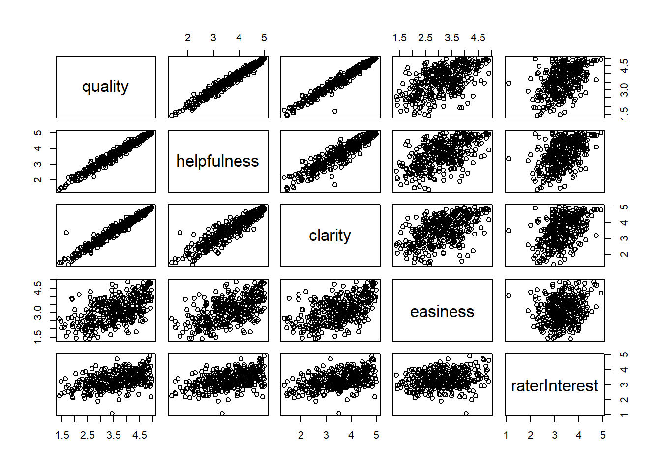
Based on the scatterplot, quality appears to be positive related to helpfulness and clarity. There’s more variablity in results for easiness and aterInterest.
Warning in model.response(mf, "numeric"): using type = "numeric" with a factor
response will be ignoredWarning in Ops.ordered(y, z$residuals): '-' is not meaningful for ordered
factors
Call:
lm(formula = tv ~ hi, data = student.survey)
Residuals:
Min 1Q Median 3Q Max
-8.600 -3.790 -1.167 2.408 27.746
Coefficients:
Estimate Std. Error t value Pr(>|t|)
(Intercept) 20.200 6.175 3.271 0.0018 **
hi -3.909 1.849 -2.114 0.0388 *
---
Signif. codes: 0 '***' 0.001 '**' 0.01 '*' 0.05 '.' 0.1 ' ' 1
Residual standard error: 6.528 on 58 degrees of freedom
Multiple R-squared: 0.07156, Adjusted R-squared: 0.05555
F-statistic: 4.471 on 1 and 58 DF, p-value: 0.03879
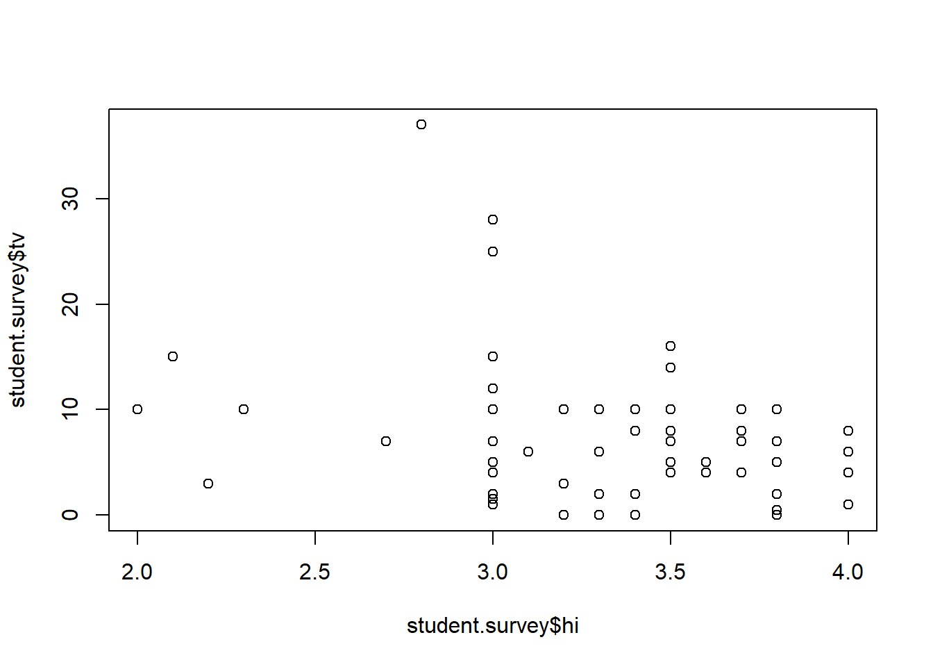
The summary above shows there is a statistically signifcate relationship between high school GPA and the number of TV hours watched per week.
---
title: 'Homework #3'
author: "Kalimah Muhammad"
date: "10/31/2022"
desription: "Regression Models"
format:
html:
toc: true
code-fold: true
code-copy: true
code-tools: true
categories:
- hw3
- Kalimah Muhammad
---
```{r}
#| label: setup
#| warning: false
library(tidyverse)
library(dplyr)
library(ggplot2)
library(alr4)
library(smss)
knitr::opts_chunk$set(echo = TRUE)
```
## Question 1: United Nations
```{r}
data(UN11) #load United Nations data
```
### 1.1.1
The predictor variable is ppgdp (the gross national product per person in USD) and the response or outcome variable in fertility (the birth rate per 1000 females).
### 1.1.2
```{r}
ggplot(UN11, aes(x=ppgdp, y=fertility))+ geom_point()
```
Fertility has the most variability at zero gross national product per person (ppgdp) where countries range from birthrate of 1 to 7 per 1000 females. There is a sharp decline thereafter where the fertility rate is consistently 3 or under and hovers between slightly above 2 and 1 for countries with a ppgdp above 30,000.
```{r}
plot(x=UN11$ppgdp, y=UN11$fertility)
```
Based on the plot above, there is little difference between the two plots.
### 1.1.3.
```{r}
plot(x= log(UN11$ppgdp), y=UN11$fertility)
```
Using natural logarithms, the model seems more plausible as the data becomes normalized.
## Question 2: Annual Income
### 2a.
When the British pound is used instead of the dollar, the steep of the slop minimizes.
### 2b.
THe correlation does not change when factoring in pound in lieu of the dollar.
## Question 3: Water runoff in the Sierras
Using the pairwise scatterplot, we find some pairs are better represented by a straight line than others. This seems to be common among mountain ranges with similar starting initials (i.e. of the ranges starting with "A" or those starting with "O").In each case, those pairs have a clear positive slope. Examining the percipitation by year and mountain range shows a wide range of variability with a singular outlier for each mountain range.
```{r}
data(water) #load water data
pairs(water) #plot pairs
```
```{r}
fit_water <- lm(Year~APMAM+ APSAB+ APSLAKE+ OPBPC+ OPRC+ OPSLAKE+ BSAAM, data=water) #create linear regression model based on year and mountain range
summary(fit_water) #summarize model
```
## Question 4: Professor ratings
```{r}
data("Rateprof") #load data
Rateprof%>%
  select(quality, helpfulness, clarity, easiness, raterInterest)%>%
pairs()
```
Based on the scatterplot, quality appears to be positive related to helpfulness and clarity. There's more variablity in results for easiness and aterInterest.
## Question 5: Student Survey
```{r}
data("student.survey")
fit_smss<- lm(factor(pi) ~ re, data = student.survey)
plot(x=student.survey$re, y=student.survey$pi)
```
```{r}
fit_smss2<- lm(tv ~ hi, data = student.survey)
summary(fit_smss2)
plot(x=student.survey$hi, y=student.survey$tv)
```
The summary above shows there is a statistically signifcate relationship between high school GPA and the number of TV hours watched per week.