Code
library(tidyverse)
library(readxl)
library(ggplot2)
library(stats)

knitr::opts_chunk$set(echo = TRUE)Megha Joseph
October 3, 2022
# A tibble: 725 × 6
LungCap Age Height Smoke Gender Caesarean
<dbl> <dbl> <dbl> <chr> <chr> <chr>
1 6.48 6 62.1 no male no
2 10.1 18 74.7 yes female no
3 9.55 16 69.7 no female yes
4 11.1 14 71 no male no
5 4.8 5 56.9 no male no
6 6.22 11 58.7 no female no
7 4.95 8 63.3 no male yes
8 7.32 11 70.4 no male no
9 8.88 15 70.5 no male no
10 6.8 11 59.2 no male no
# … with 715 more rowsDistribution of LungCap:
The distribution is a normal distribution. ## Answer 1 (b)
The mean of males appear higher than females.
# A tibble: 2 × 2
Smoke Mean
<chr> <dbl>
1 no 7.77
2 yes 8.65# A tibble: 2 × 2
Smoke stdev
<chr> <dbl>
1 no 2.73
2 yes 1.88
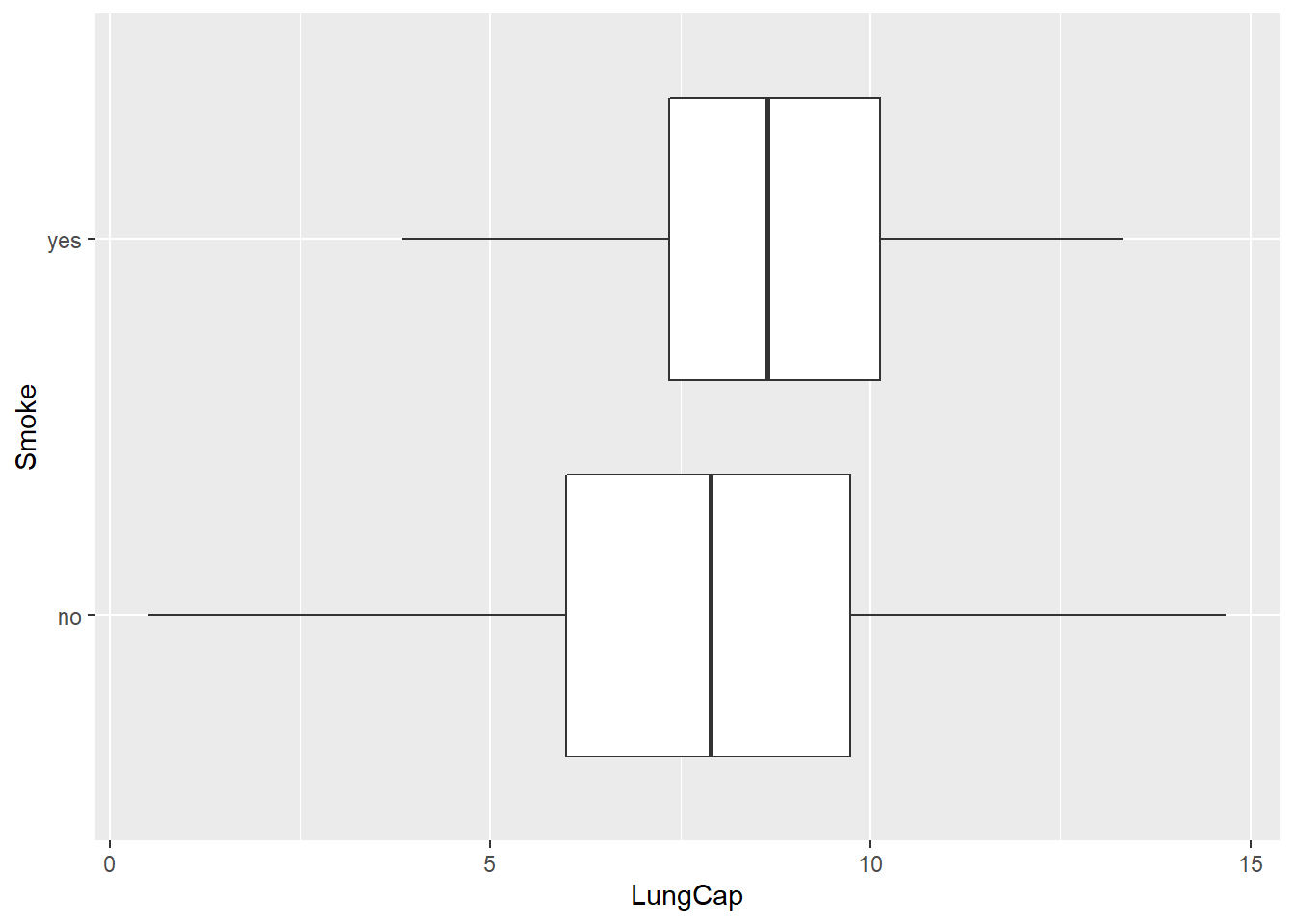
The mean of smokers is higher than the mean of non smokers and therefore it is not sensible.
[1] "numeric"`stat_bin()` using `bins = 30`. Pick better value with `binwidth`.

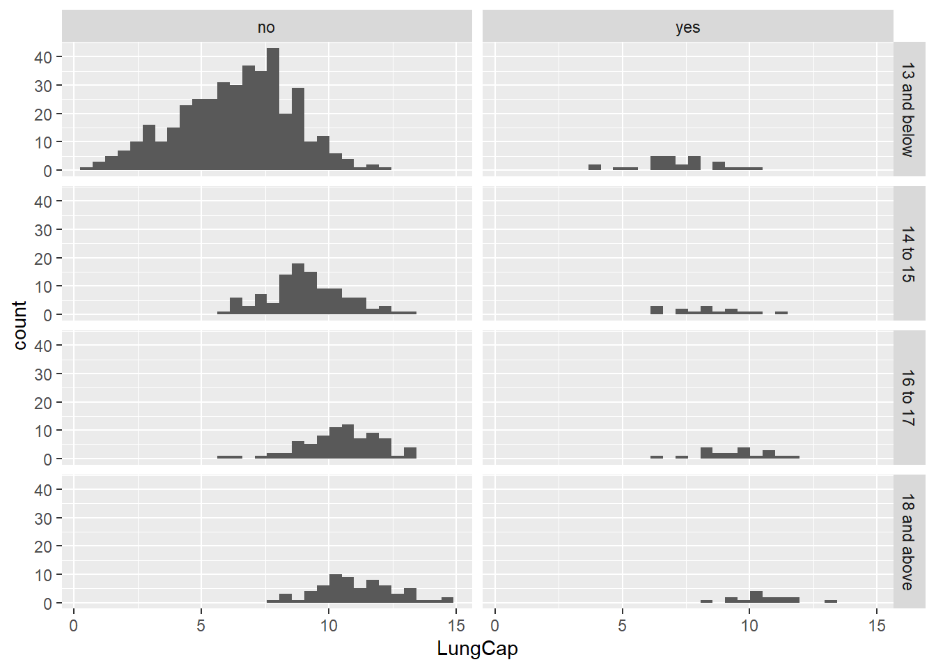
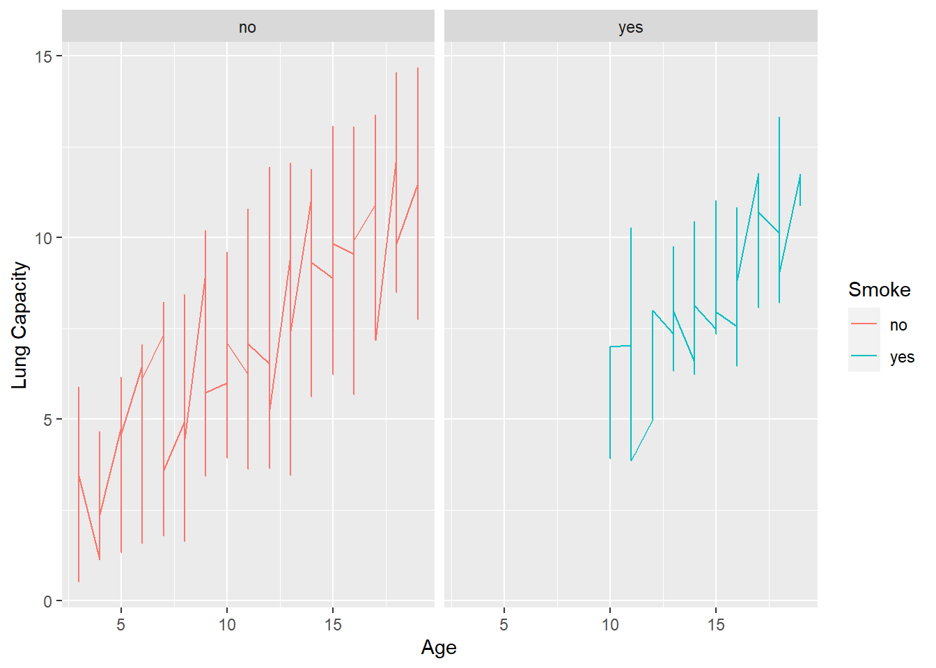
From the above results we can say that people from age group 10 and above smoke.
From the data we can see that the covariance is positive and it shows that there is a direct relationship between age and lung capacity. And the correlation is also positive, so they move in same direction. Therefore as the age increases, the lung capacity also increases that is they are directly proportional to each other.
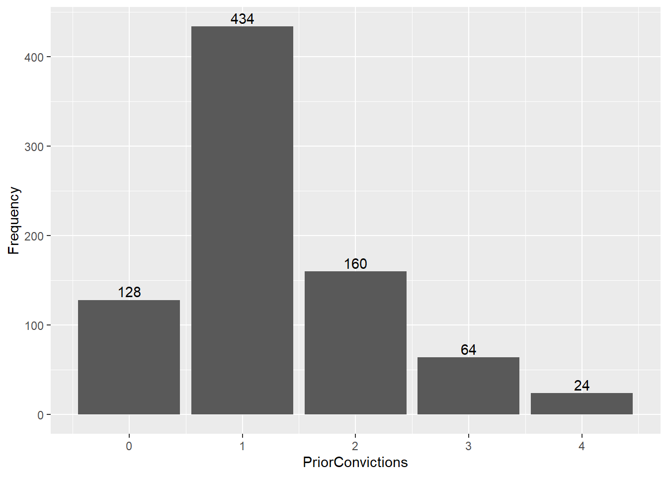
X Frequency
1 0 128
2 1 434
3 2 160
4 3 64
5 4 24 PriorConvictions Frequency
1 0 128
2 1 434
3 2 160
4 3 64
5 4 24
[1] 810[1] 0.15802469 0.53580247 0.19753086 0.07901235 0.02962963[1] 0.1975309[1] 0.6938272[1] 0.891358[1] 0.108642[1] 1.28642[1] 0.8572937[1] 0.9259016Answer
a: 19.75% b :9.38% c :89.14% d :10.86% e :1.28642 f: variance: 0.8572937 standard deviation: 0.9259016
---
title: "HOME WORK1 603"
author: "Megha Joseph"
desription: "The first homework on descriptive statistics and probability"
date: "10/03/2022"
format:
html:
toc: true
code-fold: true
code-copy: true
code-tools: true
categories:
- hw1
- descriptive statistics
- megha joseph
- probability
---
```{r}
#| label: setup
#| warning: false
library(tidyverse)
library(readxl)
library(ggplot2)
library(stats)
knitr::opts_chunk$set(echo = TRUE)
```
## Answer 1
```{r}
readD <- read_excel("_data/LungCapData.xls")
readD
```
## Answer 1 (a)
Distribution of LungCap:
```{r}
hist(readD$LungCap)
```
The distribution is a normal distribution.
## Answer 1 (b)
```{r}
boxplot(readD$LungCap ~ readD$Gender)
```
The mean of males appear higher than females.
## Answer 1 (c)
```{r}
readD%>%
  group_by(Smoke) %>%
  summarize(Mean=mean(LungCap))
readD%>%
  group_by(Smoke) %>%
  summarize(stdev=sd(LungCap))
ggplot(readD, aes(x=LungCap, y=Smoke))+geom_boxplot()
```
The mean of smokers is higher than the mean of non smokers and therefore it is not sensible.
## Answer 1 (d)
```{r}
class(readD$Age)
readD <- mutate(readD, AgeGroup = case_when(Age <= 13 ~ "13 and below",
                                            Age == 14 | Age == 15 ~ "14 to 15",
                                            Age == 16 | Age == 17 ~ "16 to 17",
                                            Age >= 18 ~ "18 and above"))
ggplot(readD, aes(x = LungCap)) +
  geom_histogram() +
  facet_grid(AgeGroup~Smoke)
```
```{r}
readD %>%
  ggplot(aes(x = Age, y = LungCap, color = Smoke)) +
  geom_line() +
  facet_wrap(vars(Smoke)) +
  labs(y = "Lung Capacity", x = "Age")
```
From the above results we can say that people from age group 10 and above smoke.
## Answer 1 (f)
```{r}
cor(readD$LungCap,readD$Age)
cov(readD$LungCap,readD$Age)
```
From the data we can see that the covariance is positive and it shows that there is a direct relationship between age and lung capacity. And the correlation is also positive, so they move in same direction. Therefore as the age increases, the lung capacity also increases that is they are directly proportional to each other.
## Answer 2
```{r}
X<-c(0, 1, 2, 3, 4)
Frequency<-c(128, 434, 160, 64, 24)
C<- data.frame(X, Frequency)
C
C<-rename(C, PriorConvictions=X)
C
#visualizing df using bar chart
ggplot(C, aes(x=PriorConvictions, y=Frequency))+geom_bar(stat="identity")+geom_text(aes(label = Frequency), vjust = -.3)
#There are 810 obs in df
sum(Frequency)
```
```{r}
PO<-Frequency/810
PO
#A
# P(x=2)=160/810
160/810
#B
#P(x<2)=P(0)+P(1)
(128+434)/810
#C
#P(x<=2)=P(0)+P(1)+P(2)
(128+434+160)/810
#D
#1-P(above)
1-((128+434+160)/810)
#E
#Expected value=sum of probabilities*each value (0, 1, 2, 3 or 4)
weighted.mean(X, PO)
#F
#Calculating the Variance using the formula for variance
(sum(Frequency*((X-1.28642)^2)))/(sum(Frequency)-1)
#Calculating the sample standard deviation from the variance
sqrt(0.8572937)
```
Answer
a: 19.75%
b :9.38%
c :89.14%
d :10.86%
e :1.28642
f: variance: 0.8572937
standard deviation: 0.9259016